Note
This tutorial was generated from a Jupyter notebook that can be accessed here.
Cost function for manifold topology assessment and optimization
In this tutorial, we present the cost function from the analysis module which distills information from the normalized variance derivative into a single number. The cost function can be used for low-dimensional manifold topology assessment and manifold optimization.
We import the necessary modules:
from PCAfold import preprocess
from PCAfold import reduction
from PCAfold import analysis
from PCAfold import utilities
from PCAfold import manifold_informed_backward_variable_elimination as BVE
import numpy as np
import time
and we set some initial parameters:
save_filename = None
random_seed = 100
Upload a combustion data set
A data set representing combustion of syngas in air generated from steady laminar flamelet model using Spitfire and a chemical mechanism by Hawkes et al. is used as a demo data set.
We begin by importing the data set composed of the original state space variables, \(\mathbf{X}\), and the corresponding source terms, \(\mathbf{S_X}\):
X = np.genfromtxt('data-state-space.csv', delimiter=',')
S_X = np.genfromtxt('data-state-space-sources.csv', delimiter=',')
X_names = ['T', 'H2', 'O2', 'O', 'OH', 'H2O', 'H', 'HO2', 'CO', 'CO2', 'HCO']

(n_observations, n_variables) = np.shape(X)
Generate low-dimensional manifolds using PCA
Below, we generate two- and three-dimensional projections of the original data set from PCA for further assessment.
pca_X_2D = reduction.PCA(X, scaling='auto', n_components=2)
Z_2D = pca_X_2D.transform(X)
S_Z_2D = pca_X_2D.transform(S_X, nocenter=True)
pca_X_3D = reduction.PCA(X, scaling='auto', n_components=3)
Z_3D = pca_X_3D.transform(X)
S_Z_3D = pca_X_3D.transform(S_X, nocenter=True)
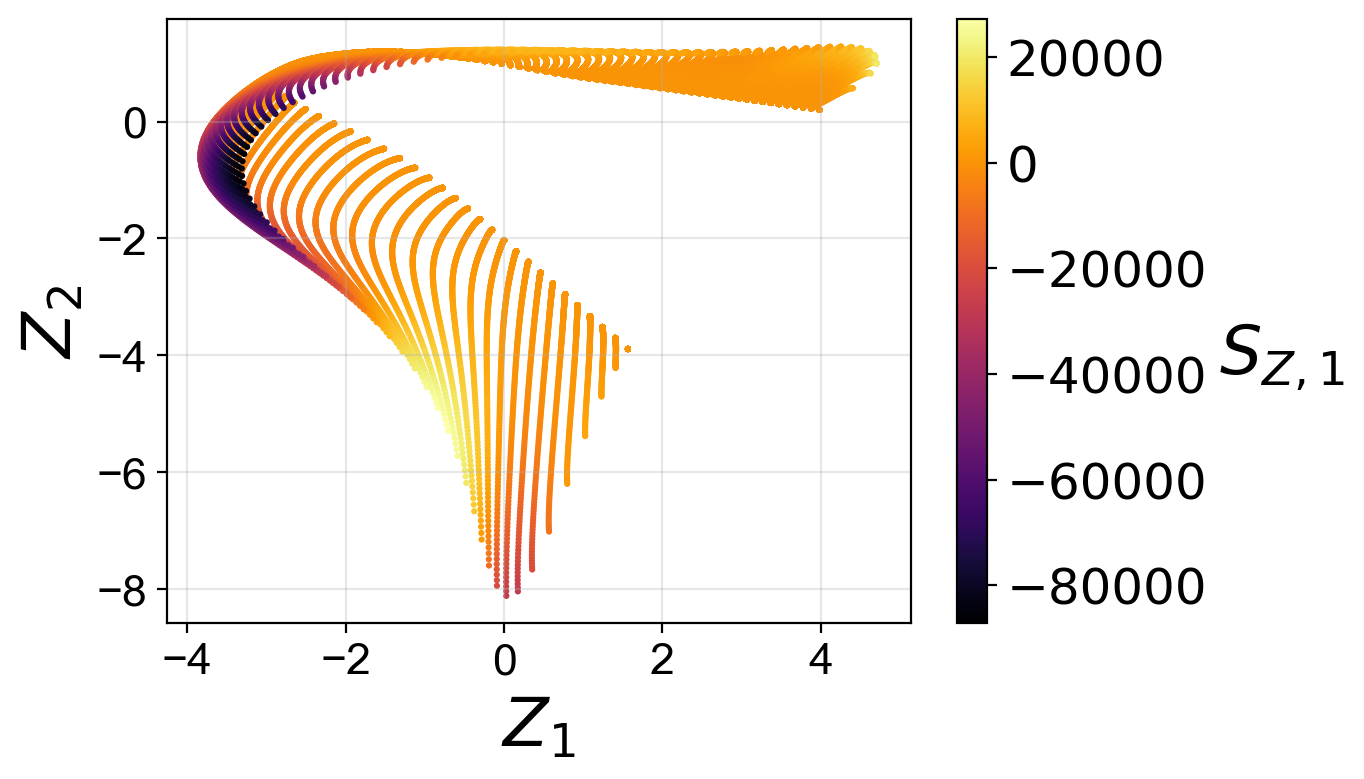
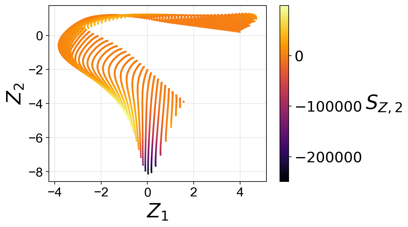
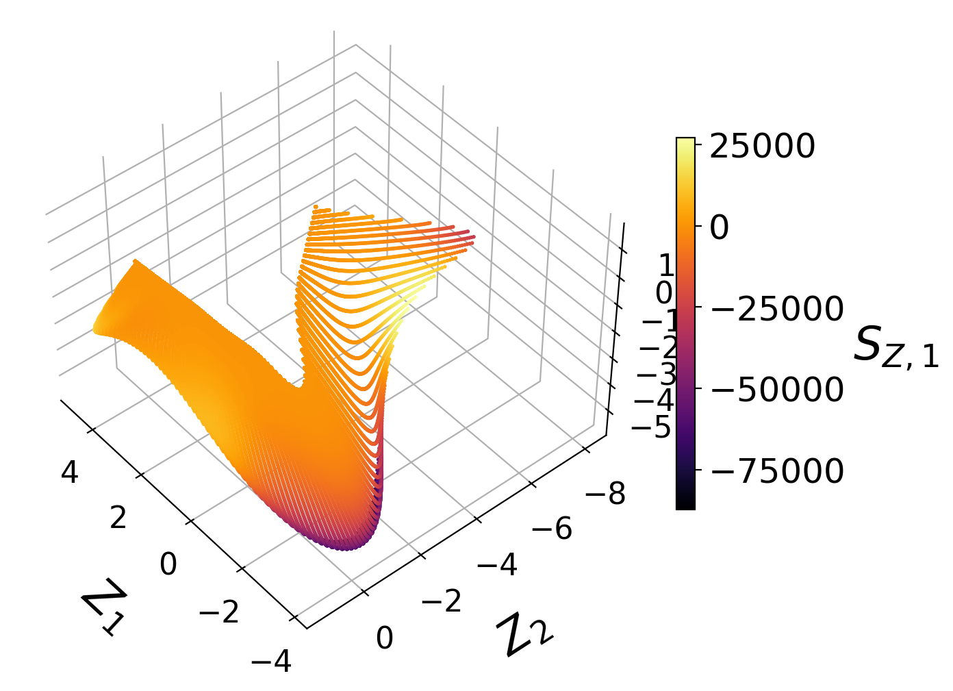
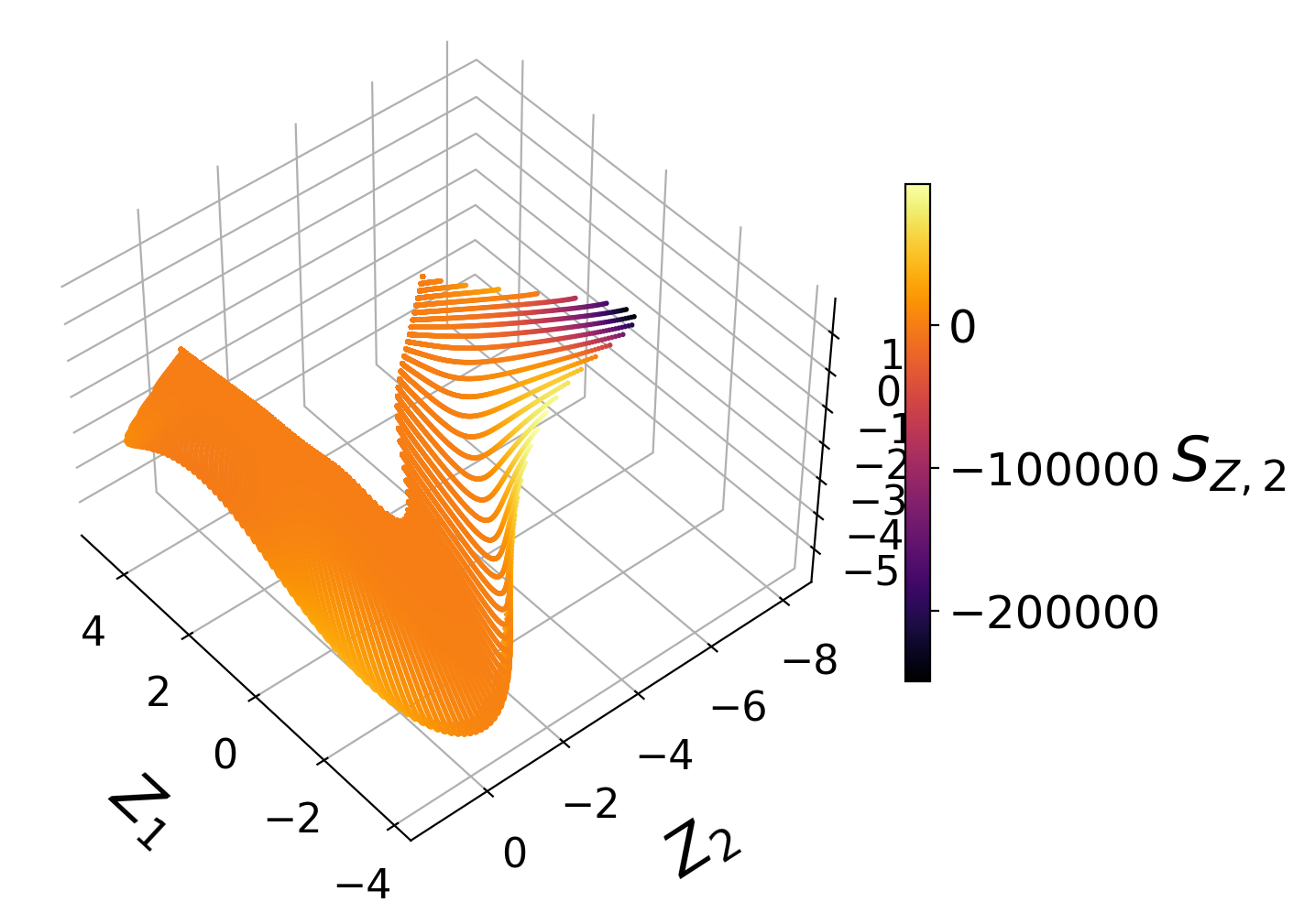
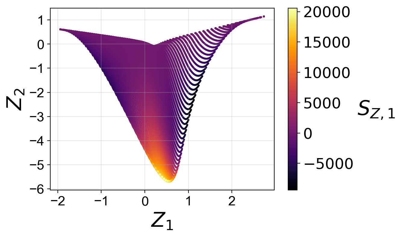
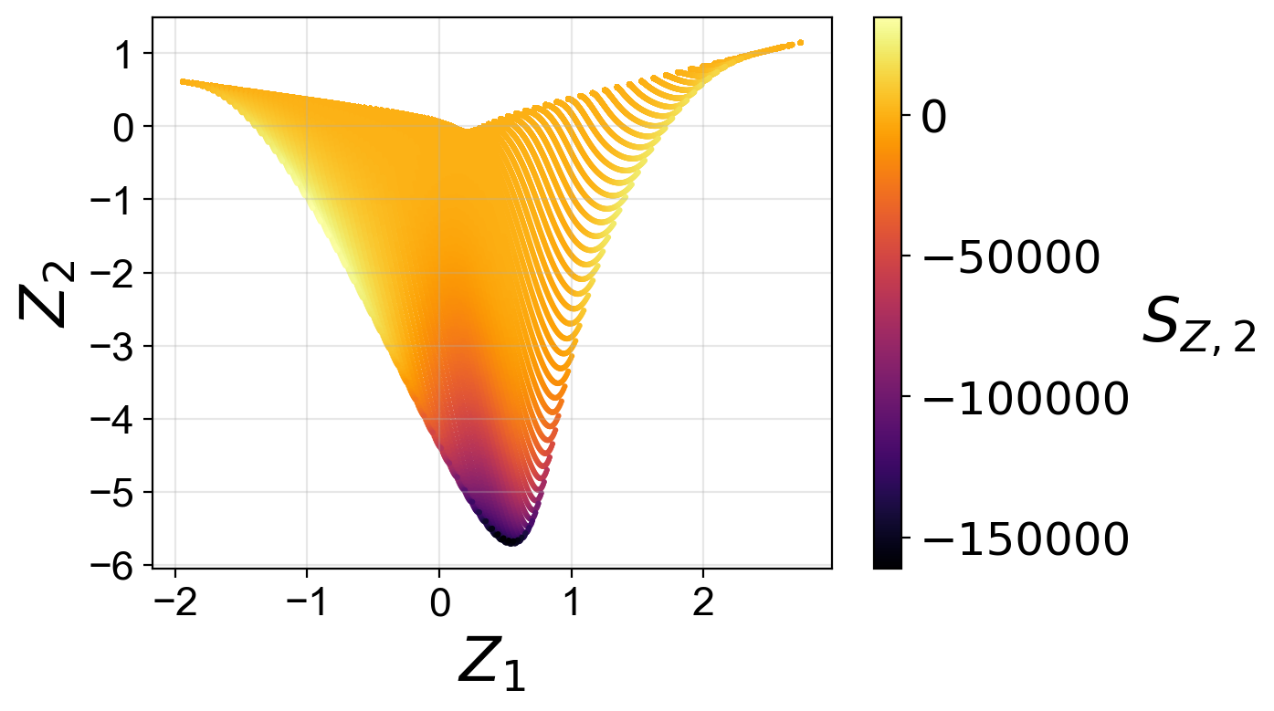
We visualize the generated manifolds:
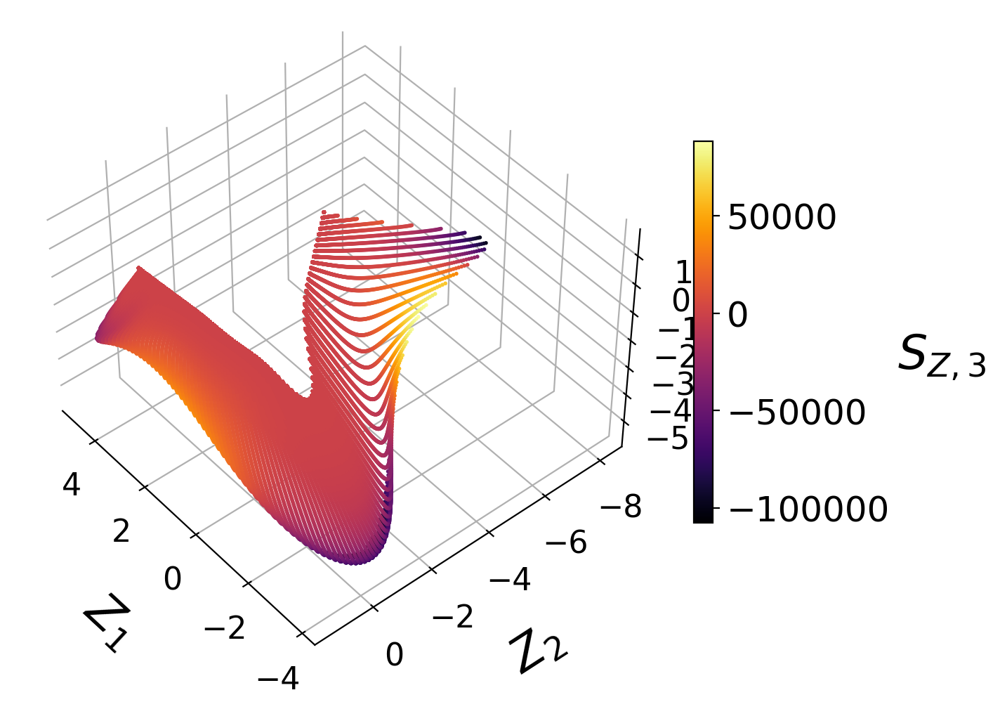
Manifold assessment using the cost function
We are going to compute the cost function for the PC source terms as the target dependent variables.
We specify the penalty function to use:
penalty_function = 'log-sigma-over-peak'
and the bandwidth values, \(\sigma\), for normalized variance derivative computation:
bandwidth_values = np.logspace(-7, 3, 50)
We specify the cost function’s hyper-parameters, the power \(r\) and the vertical shift \(b\). Increasing the power parameter allows for a stronger penalty for non-uniqueness and increasing the vertical shift parameter allows for a stronger penalty for small feature sizes.
power = 1
vertical_shift = 1
We sample the dataset to decrease the computational time of this tutorial:
sample_random = preprocess.DataSampler(np.zeros((n_observations,)).astype(int), random_seed=random_seed, verbose=False)
(idx_sample, _) = sample_random.random(50)
We create lists of the target dependent variables names:
depvar_names_2D = ['SZ' + str(i) for i in range(1,3)]
depvar_names_3D = ['SZ' + str(i) for i in range(1,4)]
and we begin with computing the normalized variance derivative for the two-dimensional PCA projection:
variance_data_2D = analysis.compute_normalized_variance(Z_2D[idx_sample,:],
                                                        S_Z_2D[idx_sample,:],
                                                        depvar_names=depvar_names_2D,
                                                        bandwidth_values=bandwidth_values)
The associated costs are computed from the generated object of the VarianceData class. With the norm=None we do not normalize the costs over all target variables (in this case the PC source terms), instead the output will give us the individual costs for each target variable.
costs_2D = analysis.cost_function_normalized_variance_derivative(variance_data_2D,
                                                                 penalty_function=penalty_function,
                                                                 power=power,
                                                                 vertical_shift=vertical_shift,
                                                                 norm=None)
We can print the individual costs:
for i, variable in enumerate(depvar_names_2D):
    print(variable + ':\t' + str(round(costs_2D[i],3)))
SZ1:        4.238
SZ2:        1.567
Finally, we repeat the cost function computation for the three-dimensional PCA projection:
variance_data_3D = analysis.compute_normalized_variance(Z_3D[idx_sample,:],
                                                        S_Z_3D[idx_sample,:],
                                                        depvar_names=depvar_names_3D,
                                                        bandwidth_values=bandwidth_values)
costs_3D = analysis.cost_function_normalized_variance_derivative(variance_data_3D,
                                                                 penalty_function=penalty_function,
                                                                 power=power,
                                                                 vertical_shift=verical_shift,
                                                                 norm=None)
and we print the individual costs:
for i, variable in enumerate(depvar_names_3D):
    print(variable + ':\t' + str(round(costs_3D[i],3)))
SZ1:        1.157
SZ2:        1.23
SZ3:        1.422
The cost function provides us information about the quality of the low-dimensional data projection with respect to target dependent variables, which in this case were the PC source terms. A higher cost indicates a worse manifold topology. The two topological aspects that the cost function takes into account are non-uniqueness and feature sizes.
We observe that individual costs are higher for the two-dimensional than for the three-dimensional PCA projection. This can be understood from our visualization of the manifolds, where we have seen a significant overlap affecting the first PC source term in particular. With the third manifold parameter added in the three-dimensional projection, the projection quality improves and the costs drop.
Moreover, for the two-dimensional PCA projection, the cost associated with the first PC source term is higher than the cost associated with the second PC source term. This can also be understood by comparing the two-dimensional projections colored by \(S_{Z, 1}\) and by \(S_{Z, 2}\). The high magnitudes of \(S_{Z, 1}\) values occur at the location where the manifold exhibits overlap, while the same overlap does not affect the \(S_{Z, 2}\) values to the same extent.
Manifold optimization using the cost function
The utilities.manifold_informed_backward_variable_elimination function implements an iterative feature selection algorithm that uses the cost function as an objective function. The algorithm selects an optimal subset of the original state variables that result in an optimized PCA manifold topology. Below, we demonstrate the algorithm on a 10% sample of the original data. The data is sampled to speed-up the calculations for the purpose of this demonstration. In real applications it is recommended to use the full data set.
Sample the original data:
sample_random = preprocess.DataSampler(np.zeros((n_observations,)).astype(int), random_seed=100, verbose=False)
(idx_sample, _) = sample_random.random(10)

sampled_X = X[idx_sample,:]
sampled_S_X = S_X[idx_sample,:]
Specify the target variables to assess on the manifold (we will also add the PC source terms to the target variables by setting add_transformed_source=True). In this case we take the temperature, $T$, and several important chemical species mass fractions: \(H_2\), \(O_2\), \(H_2O\), \(CO\) and \(CO_2\):
target_variables = sampled_X[:,[0,1,2,5,8,9]]
Set the norm to take over all target dependent variables:
norm = 'cumulative'
Set the target manifold dimensionality:
q = 2
Run the algorithm:
_, selected_variables, _, _ = BVE(sampled_X,
                                  sampled_S_X,
                                  X_names,
                                  scaling='auto',
                                  bandwidth_values=bandwidth_values,
                                  target_variables=target_variables,
                                  add_transformed_source=True,
                                  target_manifold_dimensionality=q,
                                  penalty_function=penalty_function,
                                  power=power,
                                  vertical_shift=vertical_shift,
                                  norm=norm,
                                  verbose=True)
With verbose=True we will see additional information on costs at each iteration:
Iteration No.4
Currently eliminating variable from the following list:
['T', 'H2', 'O2', 'O', 'OH', 'H2O', 'H', 'CO2']
    Currently eliminated variable: T
    Running PCA for a subset:
    H2, O2, O, OH, H2O, H, CO2
    Cost:   11.4539
    WORSE
    Currently eliminated variable: H2
    Running PCA for a subset:
    T, O2, O, OH, H2O, H, CO2
    Cost:   13.4908
    WORSE
    Currently eliminated variable: O2
    Running PCA for a subset:
    T, H2, O, OH, H2O, H, CO2
    Cost:   14.8488
    WORSE
    Currently eliminated variable: O
    Running PCA for a subset:
    T, H2, O2, OH, H2O, H, CO2
    Cost:   12.6549
    WORSE
    Currently eliminated variable: OH
    Running PCA for a subset:
    T, H2, O2, O, H2O, H, CO2
    Cost:   10.0785
    SAME OR BETTER
    Currently eliminated variable: H2O
    Running PCA for a subset:
    T, H2, O2, O, OH, H, CO2
    Cost:   10.7182
    WORSE
    Currently eliminated variable: H
    Running PCA for a subset:
    T, H2, O2, O, OH, H2O, CO2
    Cost:   11.8644
    WORSE
    Currently eliminated variable: CO2
    Running PCA for a subset:
    T, H2, O2, O, OH, H2O, H
    Cost:   10.9898
    WORSE

    Variable OH is removed.
    Cost:   10.0785

    Iteration time: 0.8 minutes.
Finally, we generate the PCA projection of the optimized subset of the original data set:
pca_X_optimized = reduction.PCA(X[:,selected_variables], scaling='auto', n_components=2)
Z_optimized = pca_X_optimized.transform(X[:,selected_variables])
S_Z_optimized = pca_X_optimized.transform(S_X[:,selected_variables], nocenter=True)
From the plots above, we observe that the optimized two-dimensional PCA projection exhibits much less overlap compared to the two-dimensional PCA projection that we computed earlier using the full data set.
Below, we compute the costs for the two PC source terms again for this optimized projection:
variance_data_optimized = analysis.compute_normalized_variance(Z_optimized,
                                                               S_Z_optimized,
                                                               depvar_names=depvar_names_2D,
                                                               bandwidth_values=bandwidth_values)
costs_optimized = analysis.cost_function_normalized_variance_derivative(variance_data_optimized,
                                                                        penalty_function=penalty_function,
                                                                        power=power,
                                                                        vertical_shift=vertical_shift,
                                                                        norm=None)
for i, variable in enumerate(depvar_names_2D):
    print(variable + ':\t' + str(round(costs_optimized[i],3)))
SZ1:        1.653
SZ2:        1.179
We note that the costs for the two PC source terms are lower than the costs that we computed earlier using the full data set to generate the PCA projection.