Module: reduction#

The reduction module contains functions for performing Principal Component Analysis (PCA).

Note

The format for the user-supplied input data matrix \(\mathbf{X} \in \mathbb{R}^{N \times Q}\), common to all modules, is that \(N\) observations are stored in rows and \(Q\) variables are stored in columns. Since typically \(N \gg Q\), the initial dimensionality of the data set is determined by the number of variables, \(Q\).

\[\begin{split}\mathbf{X} = \begin{bmatrix} \vdots & \vdots & & \vdots \\ X_1 & X_2 & \dots & X_{Q} \\ \vdots & \vdots & & \vdots \\ \end{bmatrix}\end{split}\]

The general agreement throughout this documentation is that \(i\) will index observations and \(j\) will index variables.

The representation of the user-supplied data matrix in PCAfold is the input parameter X, which should be of type numpy.ndarray and of size (n_observations,n_variables).

Principal Component Analysis#

Class `PCA`#

class PCAfold.reduction.PCA(X, scaling='std', n_components=0, use_eigendec=True, nocenter=False)#

Enables performing Principal Component Analysis (PCA) of the original data set, \(\mathbf{X}\). For more detailed information on the theory of PCA the user is referred to [Jolliffe02].

Two options for performing PCA are implemented:

Eigendecomposition of the covariance matrix Set `use_eigendec=True` (default)	Singular Value Decomposition (SVD) Set `use_eigendec=False`
Centering and scaling (as per `preprocess.center_scale` function): If `nocenter=False`: \(\mathbf{X_{cs}} = (\mathbf{X} - \mathbf{C}) \cdot \mathbf{D}^{-1}\) If `nocenter=True`: \(\mathbf{X_{cs}} = \mathbf{X} \cdot \mathbf{D}^{-1}\)
Eigendecomposition of the covariance matrix \(\mathbf{S}\)	SVD: \(\mathbf{X_{cs}} = \mathbf{U} \mathbf{\Sigma} \mathbf{V}^{\mathbf{T}}\)
Modes: Eigenvectors \(\mathbf{A}\)	Modes: \(\mathbf{A} = \mathbf{V}\)
Amplitudes: Eigenvalues \(\mathbf{L}\)	Amplitudes: \(\mathbf{L} = diag(\mathbf{\Sigma})\)

Note: For simplicity, we will from now on refer to \(\mathbf{A}\) as the matrix of eigenvectors and to \(\mathbf{L}\) as the vector of eigenvalues, irrespective of the method used to perform PCA.

Covariance matrix is computed at the class initialization as:

\[\mathbf{S} = \frac{1}{N-1} \mathbf{X_{cs}}^{\mathbf{T}} \mathbf{X_{cs}}\]

where \(N\) is the number of observations in the original data set, \(\mathbf{X}\).

Loadings matrix, \(\mathbf{l}\), is computed at the class initialization such that the element \(\mathbf{l}_{ij}\) is the corresponding scaled element of the eigenvectors matrix, \(\mathbf{A}_{ij}\):

\[\mathbf{l}_{ij} = \frac{\mathbf{A}_{ij} \sqrt{\mathbf{L}_j}}{\sqrt{\mathbf{S}_{ii}}}\]

where \(\mathbf{L}_j\) is the \(j^{th}\) eigenvalue and \(\mathbf{S}_{ii}\) is the \(i^{th}\) element on the diagonal of the covariance matrix, \(\mathbf{S}\).

The variance accounted for in each individual variable by the first \(q\) PCs, \(\mathbf{t_q}\), is computed at the class initialization:

\[\mathbf{t}_{\mathbf{q}i} = \sum_{j=1}^{q} \Bigg( \frac{\mathbf{A}_{ij} \sqrt{\mathbf{L}_j}}{ s_i } \Bigg)^2\]

where \(q\) is the number of retained principal components and \(s_i\) is the standard deviation of the \(i^{th}\) variable in the data set.

Example:

from PCAfold import PCA
import numpy as np

# Generate dummy data set:
X = np.random.rand(100,20)

# Instantiate PCA class object:
pca_X = PCA(X, scaling='none', n_components=2, use_eigendec=True, nocenter=False)

# Access the eigenvectors:
A = pca_X.A

# Access the eigenvalues:
L = pca_X.L

# Access the loadings:
l = pca_X.loadings

# Access the variance accounted for each variable:
tq = pca_X.tq

Parameters:

X – numpy.ndarray specifying the original data set, \(\mathbf{X}\). It should be of size (n_observations,n_variables).
scaling – str specifying the scaling methodology. It can be one of the following: 'none', '', 'auto', 'std', 'pareto', 'vast', 'range', '0to1', '-1to1', 'level', 'max', 'variance', 'median', 'poisson', 'vast_2', 'vast_3', 'vast_4'.
n_components – (optional) int specifying the number of retained principal components, \(q\). If set to 0 all PCs are retained. It should be a non-negative number.
use_eigendec –
(optional) bool specifying the method for obtaining eigenvalues and eigenvectors:
- use_eigendec=True uses eigendecomposition of the covariance matrix (from numpy.linalg.eigh)
- use_eigendec=False uses Singular Value Decomposition (SVD) (from scipy.linalg.svd)
nocenter – (optional) bool specifying whether the data original data set should be centered by mean.

Attributes:

n_components - (can be re-set) number of retained principal components, \(q\).
n_components_init - (read only) number of retained principal components, \(q\), with which PCA class object was initialized.
scaling - (read only) scaling criteria with which PCA class object was initialized.
n_variables - (read only) number of variables of the original data set on which PCA class object was initialized.
X_cs - (read only) centered and scaled data set \(\mathbf{X_{cs}}\).
X_center - (read only) vector of centers, \(\mathbf{C}\), applied on the original data set \(\mathbf{X}\).
X_scale - (read only) vector of scales, \(\mathbf{D}\), applied on the original data set \(\mathbf{X}\).
S - (read only) covariance matrix, \(\mathbf{S}\).
L - (read only) vector of eigenvalues, \(\mathbf{L}\).
A - (read only) matrix of eigenvectors, \(\mathbf{A}\), (vectors are stored in columns, rows correspond to weights).
loadings - (read only) loadings, \(\mathbf{l}\), (vectors are stored in columns, rows correspond to weights).
tq - (read only) variance accounted for in each individual variable, \(\mathbf{t_q}\).
tq - (read only) variance accounted for in each individual variable in each PC, \(\mathbf{t_{q,j}}\).

PCAfold.reduction.PCA.transform(self, X, nocenter=False)#

Transforms any original data set, \(\mathbf{X}\), to a new truncated basis, \(\mathbf{A}_q\), identified by PCA. It computes the \(q\) first principal components, \(\mathbf{Z}_q\), given the original data.

If nocenter=False:

\[\mathbf{Z}_q = (\mathbf{X} - \mathbf{C}) \cdot \mathbf{D}^{-1} \cdot \mathbf{A}_q\]

If nocenter=True:

\[\mathbf{Z}_q = \mathbf{X} \cdot \mathbf{D}^{-1} \cdot \mathbf{A}_q\]

Here \(\mathbf{C}\) and \(\mathbf{D}\) are centers and scales computed during PCA class initialization and \(\mathbf{A}_q\) is the matrix of \(q\) first eigenvectors extracted from \(\mathbf{A}\).

Warning

Set nocenter=True only if you know what you are doing.

One example when nocenter should be set to True is when transforming chemical source terms, \(\mathbf{S_X}\), to principal components space (as per [SP09]) to obtain sources of principal components, \(\mathbf{S_Z}\). In that case \(\mathbf{X} = \mathbf{S_X}\) and the transformation should be performed without centering:

\[\mathbf{S}_{\mathbf{Z}, q} = \mathbf{S_X} \cdot \mathbf{D}^{-1} \cdot \mathbf{A}_q\]

Example:

from PCAfold import PCA
import numpy as np

# Generate dummy data set:
X = np.random.rand(100,20)

# Instantiate PCA class object:
pca_X = PCA(X, scaling='none', n_components=2, use_eigendec=True, nocenter=False)

# Calculate the principal components:
principal_components = pca_X.transform(X)

Parameters:

X – numpy.ndarray specifying the data set \(\mathbf{X}\) to transform. It should be of size (n_observations,n_variables). Note that it does not need to be the same data set that was used to construct the PCA class object. It could for instance be a function of that data set. By default, this data set will be pre-processed with the centers and scales computed on the data set used when constructing the PCA object.
nocenter – (optional) bool specifying whether PCA.X_center centers should be applied to center the data set before transformation. If nocenter=True centers will not be applied on the data set.

Returns:

principal_components - numpy.ndarray specifying the \(q\) first principal components \(\mathbf{Z}_q\). It has size (n_observations,n_components).

PCAfold.reduction.PCA.reconstruct(self, principal_components, nocenter=False)#

Calculates rank-\(q\) reconstruction of the data set from the \(q\) first principal components, \(\mathbf{Z}_q\).

If nocenter=False:

\[\mathbf{X_{rec}} = \mathbf{Z}_q \mathbf{A}_q^{\mathbf{T}} \cdot \mathbf{D} + \mathbf{C}\]

If nocenter=True:

\[\mathbf{X_{rec}} = \mathbf{Z}_q \mathbf{A}_q^{\mathbf{T}} \cdot \mathbf{D}\]

Here \(\mathbf{C}\) and \(\mathbf{D}\) are centers and scales computed during PCA class initialization and \(\mathbf{A}_q\) is the matrix of \(q\) first eigenvectors extracted from \(\mathbf{A}\).

Warning

Set nocenter=True only if you know what you are doing.

One example when nocenter should be set to True is when reconstructing chemical source terms, \(\mathbf{S_X}\), (as per [SP09]) from the \(q\) first sources of principal components, \(\mathbf{S}_{\mathbf{Z}, q}\). In that case \(\mathbf{Z}_q = \mathbf{S}_{\mathbf{Z}, q}\) and the reconstruction should be performed without uncentering:

\[\mathbf{S_{X, rec}} = \mathbf{S}_{\mathbf{Z}, q} \mathbf{A}_q^{\mathbf{T}} \cdot \mathbf{D}\]

Example:

from PCAfold import PCA
import numpy as np

# Generate dummy data set:
X = np.random.rand(100,20)

# Instantiate PCA class object:
pca_X = PCA(X, scaling='none', n_components=2, use_eigendec=True, nocenter=False)

# Calculate the principal components:
principal_components = pca_X.transform(X)

# Calculate the reconstructed variables:
X_rec = pca_X.reconstruct(principal_components)

Parameters:

principal_components – numpy.ndarray of \(q\) first principal components, \(\mathbf{Z}_q\). It should be of size (n_observations,n_variables).
nocenter – (optional) bool specifying whether PCA.X_center centers should be applied to un-center the reconstructed data set. If nocenter=True centers will not be applied on the reconstructed data set.

Returns:

X_rec - rank-\(q\) reconstruction of the original data set.

PCAfold.reduction.PCA.get_weights_dictionary(self, variable_names, pc_index, n_digits=10)#

Creates a dictionary where keys are the names of the variables in the original data set \(\mathbf{X}\) and values are the eigenvector weights corresponding to the principal component selected by pc_index. This function helps in accessing weight value for a specific variable and for a specific PC.

Example:

from PCAfold import PCA
import numpy as np

# Generate dummy data set:
X = np.random.rand(100,5)

# Generate dummy variables names:
variable_names = ['A1', 'A2', 'A3', 'A4', 'A5']

# Instantiate PCA class object:
pca_X = PCA(X, scaling='auto', n_components=0, use_eigendec=True, nocenter=False)

# Create a dictionary for PC-1 weights:
PC1_weights_dictionary = pca_X.get_weights_dictionary(variable_names, 0, n_digits=8)

The code above will create a dictionary:

{'A1': 0.63544443,
 'A2': -0.39500424,
 'A3': -0.28819465,
 'A4': 0.57000796,
 'A5': 0.17949037}

Eigenvector weight for a specific variable can then be accessed by:

PC1_weights_dictionary['A3']

Parameters:

variable_names – list of str specifying names for all variables in the original data set, \(\mathbf{X}\).
pc_index – non-negative int specifying the index of the PC to create the dictionary for. Set pc_index=0 if you want to look at the first PC.
n_digits – (optional) non-negative int specifying how many digits should be kept in rounding the eigenvector weights.

Returns:

weights_dictionary - dict of variable names as keys and selected eigenvector weights as values.

PCAfold.reduction.PCA.u_scores(self, X)#

Calculates the U-scores (principal components):

\[\mathbf{U_{scores}} = \mathbf{X_{cs}} \mathbf{A}_q\]

This function is equivalent to PCA.transform.

Example:

from PCAfold import PCA
import numpy as np

# Generate dummy data set:
X = np.random.rand(100,20)

# Instantiate PCA class object:
pca_X = PCA(X, scaling='auto', n_components=10, use_eigendec=True, nocenter=False)

# Calculate the U-scores:
u_scores = pca_X.u_scores(X)

Parameters:

X – data set to transform. Note that it does not need to be the same data set that was used to construct the PCA object. It could for instance be a function of that data set. By default, this data set will be pre-processed with the centers and scales computed on the data set used when constructing the PCA object.

Returns:

u_scores - U-scores (principal components).

PCAfold.reduction.PCA.w_scores(self, X)#

Calculates the W-scores which are the principal components scaled by the inverse square root of the corresponding eigenvalue:

\[\mathbf{W_{scores}} = \frac{\mathbf{Z}_q}{\sqrt{\mathbf{L_q}}}\]

where \(\mathbf{L_q}\) are the \(q\) first eigenvalues extracted from \(\mathbf{L}\). The W-scores are still uncorrelated and have variances equal unity.

Example:

from PCAfold import PCA
import numpy as np

# Generate dummy data set:
X = np.random.rand(100,20)

# Instantiate PCA class object:
pca_X = PCA(X, scaling='auto', n_components=10, use_eigendec=True, nocenter=False)

# Calculate the W-scores:
w_scores = pca_X.w_scores(X)

Parameters:

Returns:

w_scores - W-scores (scaled principal components).

PCAfold.reduction.PCA.calculate_r2(self, X)#

Calculates coefficient of determination, \(R^2\), values for the rank-\(q\) reconstruction, \(\mathbf{X_{rec}}\), of the original data set, \(\mathbf{X}\):

\[R^2 = 1 - \frac{\sum_{i=1}^N (\mathbf{X}_i - \mathbf{X_{rec}}_i)^2}{\sum_{i=1}^N (\mathbf{X}_i - mean(\mathbf{X}_i))^2}\]

where \(\mathbf{X}_i\) is the \(i^{th}\) column of \(\mathbf{X}\), \(\mathbf{X_{rec}}_i\) is the \(i^{th}\) column of \(\mathbf{X_{rec}}\) and \(N\) is the number of observations in \(\mathbf{X}\).

If all of the eigenvalues are retained, \(R^2\) will be equal to unity.

Example:

from PCAfold import PCA
import numpy as np

# Generate dummy data set:
X = np.random.rand(100,20)

# Instantiate PCA class object:
pca_X = PCA(X, scaling='auto', n_components=10, use_eigendec=True, nocenter=False)

# Calculate the R2 values:
r2 = pca_X.calculate_r2(X)

Parameters:

X – numpy.ndarray specifying the original data set, \(\mathbf{X}\). It should be of size (n_observations,n_variables).

Returns:

r2 - numpy.ndarray specifying the coefficient of determination values \(R^2\) for the rank-\(q\) reconstruction of the original data set. It has size (n_variables,).

PCAfold.reduction.PCA.r2_convergence(self, X, n_pcs, variable_names=[], print_width=10, verbose=False, save_filename=None)#

Returns and optionally prints and/or saves to .txt file \(R^2\) values (as per PCA.calculate_r2 function) for reconstruction of the original data set \(\mathbf{X}\) as a function of number of retained principal components (PCs).

Example:

from PCAfold import PCA
import numpy as np

# Generate dummy data set:
X = np.random.rand(100,3)

# Instantiate PCA class object:
pca_X = PCA(X, scaling='auto', n_components=3)

# Compute and print convergence of R2 values:
r2 = pca_X.r2_convergence(X, n_pcs=3, variable_names=['X1', 'X2', 'X3'], print_width=10, verbose=True)

The code above will print \(R^2\) values retaining 1-3 PCs:

| n PCs      | X1         | X2         | X3         | Mean       |
| 1          | 0.17857365 | 0.53258736 | 0.49905763 | 0.40340621 |
| 2          | 0.99220888 | 0.57167479 | 0.61150487 | 0.72512951 |
| 3          | 1.0        | 1.0        | 1.0        | 1.0        |

Parameters:

X – numpy.ndarray specifying the original data set, \(\mathbf{X}\). It should be of size (n_observations,n_variables).
n_pcs – the maximum number of PCs to consider.
variable_names – (optional) list of ‘str’ specifying variable names. If not specified variables will be numbered.
print_width – (optional) width of columns printed out.
verbose – (optional) bool for printing out the table with \(R^2\) values.
save_filename – (optional) str specifying .txt save location/filename.

Returns:

r2 - matrix of size (n_pcs, n_variables) containing the \(R^2\) values for each variable as a function of the number of retained PCs.

PCAfold.reduction.PCA.set_retained_eigenvalues(self, method='SCREE GRAPH', option=None)#

Helps determine how many principal components (PCs) should be retained. The following methods are available:

'TOTAL VARIANCE' - retain the PCs whose eigenvalues account for a specific percentage of the total variance. The required number of PCs is then the smallest value of \(q\) for which this chosen percentage is exceeded. Fraction of variance can be supplied using the option parameter. For instance, set option=0.6 if you want to account for 60% variance. If variance is not supplied in the option paramter, the user will be asked for input during function execution.
'INDIVIDUAL VARIANCE' - retain the PCs whose eigenvalues are greater than the average of the eigenvalues [Kai60] or than 0.7 times the average of the eigenvalues [Jol72]. For a correlation matrix this average equals 1. Fraction of variance can be supplied using the option parameter. For instance, set option=0.6 if you want to account for 60% variance. If variance is not supplied in the option paramter, the user will be asked for input during function execution.
'BROKEN STICK' - retain the PCs according to the Broken Stick Model [Fro76].
'SCREE GRAPH' - retain the PCs using the scree graph, a plot of the eigenvalues agaist their indexes, and look for a natural break between the large and small eigenvalues.

For more detailed information on the options implemented here the user is referred to [Jolliffe02].

Example:

from PCAfold import PCA
import numpy as np

# Generate dummy data set:
X = np.random.rand(100,20)

# Instantiate PCA class object:
pca_X = PCA(X, scaling='auto')

# Compute a new ``PCA`` class object with the new number of retained components:
pca_X_new = pca_X.set_retained_eigenvalues(method='TOTAL VARIANCE', option=0.6)

# The new number of principal components that has been set:
print(pca_X_new.n_components)

This function provides a few methods to select the number of eigenvalues to be retained in the PCA reduction.

Parameters:

method – (optional) str specifying the method to use in selecting retained eigenvalues.
option – (optional) additional parameter used for the 'TOTAL VARIANCE' and 'INDIVIDUAL VARIANCE' methods. If not supplied, information will be obtained interactively.

Returns:

pca - the PCA object with the number of retained eigenvalues set on it.

PCAfold.reduction.PCA.principal_variables(self, method='B2', x=[])#

Extracts Principal Variables (PVs) from a PCA.

The following methods are currently supported:

'B4' - selects Principal Variables based on the variables contained in the eigenvectors corresponding to the largest eigenvalues [Jol72].
'B2' - selects Principal Variables based on the variables contained in the smallest eigenvalues. These are discarded and the remaining variables are used as the PVs [Jol72].
'M2' - at each iteration, each remaining variable is analyzed via PCA [Krz87]. Note: this is a very expensive method.

For more detailed information on the options implemented here the user is referred to [Jolliffe02].

Example:

from PCAfold import PCA
import numpy as np

# Generate dummy data set:
X = np.random.rand(100,20)

# Instantiate PCA class object:
pca_X = PCA(X, scaling='auto')

# Select Principal Variables (PVs) using M2 method:
principal_variables_indices = pca_X.principal_variables(method='M2', X)

Parameters:

method – (optional) str specifying the method for determining the Principal Variables (PVs).
x – (optional) data set to accompany 'M2' method. Note that this is only required for the 'M2' method.

Returns:

principal_variables_indices - a vector of indices of retained Principal Variables (PVs).

PCAfold.reduction.PCA.data_consistency_check(self, X, errors_are_fatal=False)#

Checks if the supplied data matrix X is consistent with the current PCA class object.

Example:

from PCAfold import PCA
import numpy as np

# Generate dummy data set:
X = np.random.rand(100,20)

# Instantiate PCA class object:
pca_X = PCA(X, scaling='auto', n_components=10)

# This data set will be consistent:
X_1 = np.random.rand(50,20)
is_consistent = pca_X.data_consistency_check(X_1)

# This data set will not be consistent but will not throw ValueError:
X_2 = np.random.rand(100,10)
is_consistent = pca_X.data_consistency_check(X_2)

# This data set will not be consistent and will throw ValueError:
X_3 = np.random.rand(100,10)
is_consistent = pca_X.data_consistency_check(X_3, errors_are_fatal=True)

Parameters:

X – numpy.ndarray specifying the original data set, \(\mathbf{X}\). It should be of size (n_observations,n_variables).
errors_are_fatal – (optional) bool indicating if ValueError should be raised if an incompatibility is detected.

Returns:

is_consistent - bool specifying whether or not the supplied data matrix \(\mathbf{X}\) is consistent with the PCA class object.

PCAfold.reduction.PCA.save_to_txt(self, save_filename)#

Writes the eigenvector matrix, \(\mathbf{A}\), loadings, \(\mathbf{l}\), centering, \(\mathbf{C}\), and scaling ,:math:mathbf{D}, to .txt file.

Example:

from PCAfold import PCA
import numpy as np

# Generate dummy data set:
X = np.random.rand(100,5)

# Instantiate PCA class object:
pca_X = PCA(X, scaling='auto', n_components=5)

# Save the PCA results to .txt:
pca_X.save_to_txt('pca_X_Data.txt')

Parameters:: save_filename – str specifying .txt save location/filename.

Local Principal Component Analysis#

Class `LPCA`#

class PCAfold.reduction.LPCA(X, idx, scaling='std', n_components=0, use_eigendec=True, nocenter=False, verbose=False)#

Enables performing local Principal Component Analysis (LPCA) of the original data set, \(\mathbf{X}\), partitioned into clusters.

Example:

from PCAfold import LPCA
import numpy as np

# Generate dummy data set:
X = np.random.rand(100,10)

# Generate dummy vector of cluster classifications:
idx = np.zeros((100,))
idx[50:80] = 1
idx = idx.astype(int)

# Instantiate LPCA class object:
lpca_X = LPCA(X, idx, scaling='none', n_components=2)

# Access the local covariance matrix in the first cluster:
S_k1 = lpca_X.S[0]

# Access the local eigenvectors in the first cluster:
A_k1 = lpca_X.A[0]

# Access the local eigenvalues in the first cluster:
L_k1 = lpca_X.L[0]

# Access the local principal components in the first cluster:
Z_k1 = lpca_X.principal_components[0]

# Access the local loadings in the first cluster:
l_k1 = lpca_X.loadings[0]

# Access the local variance accounted for in each individual variable in the first cluster:
tq_k1 = lpca_X.tq[0]

Parameters:

X – numpy.ndarray specifying the original data set, \(\mathbf{X}\). It should be of size (n_observations,n_variables).
idx – numpy.ndarray of cluster classifications. It should be of size (n_observations,) or (n_observations,1).
scaling – (optional) str specifying the scaling methodology. It can be one of the following: 'none', '', 'auto', 'std', 'pareto', 'vast', 'range', '0to1', '-1to1', 'level', 'max', 'variance', 'median', 'poisson', 'vast_2', 'vast_3', 'vast_4'.
n_components – (optional) int specifying the number of returned eigenvectors, eigenvalues and principal components, \(q\). If set to 0 all are returned.
use_eigendec –
(optional) bool specifying the method for obtaining eigenvalues and eigenvectors:
- use_eigendec=True uses eigendecomposition of the covariance matrix (from numpy.linalg.eigh)
- use_eigendec=False uses Singular Value Decomposition (SVD) (from scipy.linalg.svd)
nocenter – (optional) bool specifying whether data should be centered by mean.
verbose – (optional) bool for printing verbose details.

Attributes:

S - (read only) list of numpy.ndarray specifying the local covariance matrix, \(\mathbf{S}\). Each list element corresponds to the covariance matrix in a single cluster.
A - (read only) list of numpy.ndarray specifying the local eigenvectors, \(\mathbf{A}\). Each list element corresponds to eigenvectors in a single cluster.
L - (read only) list of numpy.ndarray specifying the local eigenvalues, \(\mathbf{L}\). Each list element corresponds to eigenvalues in a single cluster.
principal_components - (read only) list of numpy.ndarray specifying the local principal components, \(\mathbf{Z}\). Each list element corresponds to principal components in a single cluster.
loadings - (read only) list of numpy.ndarray specifying the local loadings, \(\mathbf{l}\). Each list element corresponds to loadings in a single cluster.
tq - (read only) list of numpy.ndarray specifying the local variance accounted for in each individual variable by the first \(q\) PCs, \(\mathbf{t_q}\). Each list element corresponds to variance metric in a single cluster.
X_reconstructed - (read only) numpy.ndarray specifying the dataset reconstructed from local PCA using the first \(q\) PCs. It has size (n_observations,n_variables).
R2 - (read only) list specifying the average coefficient of determination for each cluster reconstructed using the first \(q\) PCs. Each list element corresponds to each reconstructed cluster and is averaged over all non-constant state variables in that cluster.
idx_retained_in_clusters - (read only) list of list specifying the variables retained in each cluster. If a variable within a particular cluster becomes constant, it will be removed from this list.

PCAfold.reduction.LPCA.local_correlation(self, variable, index=0, metric='pearson', display=None, verbose=False)#

Computes a correlation in each cluster and a globally-averaged correlation between the local principal component, PC, and some specified variable, \(\phi\). The average is taken from each of the \(k\) clusters. Correlation in the \(n^{th}\) cluster is referred to as \(r_n(\mathrm{PC}, \phi)\).

This functionality has been used in [ZdybalDAlessioA+23].

Available correlation functions are:

Pearson correlation coefficient (PCC), set metric='pearson':

\[r_n(\mathrm{PC}, \phi) = \mathrm{abs} \Bigg( \frac{\sum_{i=1}^{N_n} (\mathrm{PC}_i - \overline{\mathrm{PC}}) (\phi_i - \bar{\phi})}{\sqrt{\sum_{i=1}^{N_n} (\mathrm{PC}_i - \overline{\mathrm{PC}})^2} \sqrt{\sum_{i=1}^{N_n} (\phi_i - \bar{\phi})^2}} \Bigg)\]

where \(N_n\) is the number of observations in the \(n^{th}\) cluster.

Spearman correlation coefficient (SCC), set metric='spearman'.
Distance correlation (dCor), set metric='dcor':

\[r_n(\mathrm{PC}, \phi) = \sqrt{ \frac{\mathrm{dCov}(\mathrm{PC}_n, \phi_n)}{\mathrm{dCov}(\mathrm{PC}_n, \mathrm{PC}_n) \mathrm{dCov}(\phi_n, \phi_n)} }\]

where \(\mathrm{dCov}\) is the distance covariance computed for any two variables, \(X\) and \(Y\), as:

\[\mathrm{dCov}(X,Y) = \sqrt{ \frac{1}{N^2} \sum_{i,j=1}^N x_{i,j} y_{i,j}}\]

where \(x_{i,j}\) and \(y_{i,j}\) are the elements of the double-centered Euclidean distances matrices for \(X\) and \(Y\) observations respectively. \(N\) is the total number of observations. Note, that the distance correlation computation allows \(X\) and \(Y\) to have different dimensions.

Note

The distance correlation computation requires the dcor module. You can install it through:

pip install dcor

Globally-averaged correlation metric is computed in two variants:

Weighted, where each local correlation is weighted by the size of each cluster:

\[\bar{r} = \frac{1}{N} \sum_{n=1}^k N_n r_n(\mathrm{PC}, \phi)\]

Unweighted, which computes an arithmetic average of local correlations from all clusters:

\[r = \frac{1}{k} \sum_{n=1}^k r_n(\mathrm{PC}, \phi)\]

Example:

from PCAfold import predefined_variable_bins, LPCA
import numpy as np

# Generate dummy data set:
x = np.linspace(-1,1,1000)
y = -x**2 + 1
X = np.hstack((x[:,None], y[:,None]))

# Generate dummy vector of cluster classifications:
(idx, _) = predefined_variable_bins(x, [-0.9, 0, 0.6])

# Instantiate LPCA class object:
lpca = LPCA(X, idx, scaling='none')

# Compute local Pearson correlation coefficient between PC-1 and y:
(local_correlations, weighted, unweighted) = lpca.local_correlation(y, index=0, metric='pearson', verbose=True)

With verbose=True we will see some detailed information:

PCC in cluster 1:   0.999996
PCC in cluster 2:   -0.990817
PCC in cluster 3:   0.983221
PCC in cluster 4:   0.999838

Globally-averaged weighted correlation: 0.990801
Globally-averaged unweighted correlation: 0.993468

Parameters:

variable – numpy.ndarray specifying the variable, \(\phi\), for correlation computation. It should be of size (n_observations,) or (n_observations,1) or (n_observations,n_variables) when metric='dcor'.
index – (optional) int specifying the index of the local principal component for correlation computation. Set index=0 if you want to look at the first PC.
metric – (optional) str specifying the correlation metric to use. It can be 'pearson', 'spearman' or 'dcor'.
display – (optional) str specifying the display format for the correlations. It can be 'abs', 'percent', 'abs-percent'.
verbose – (optional) bool for printing verbose details.

Returns:

local_correlations - numpy.ndarray specifying the computed correlation in each cluster. It has size (k,).
weighted - float specifying the globally-averaged weighted correlation.
unweighted - float specifying the globally-averaged unweighted correlation.

Vector Quantization Principal Component Analysis#

Class `VQPCA`#

class PCAfold.reduction.VQPCA(X, n_clusters, n_components, scaling='std', idx_init='random', max_iter=300, tolerance=None, random_state=None, verbose=False)#

Enables performing Vector Quantization with Principal Component Analysis (VQPCA).

The VQPCA algorithm was first proposed in [KL97] and its modified version that we present here was developed by [PSTS09]. VQPCA assigns observations to local clusters based on the minimum reconstruction error from PCA approximation with n_components number of Principal Components. This is an iterative procedure in which the reconstruction errors are evaluated for every observation as if that observation belonged to cluster j and next, the observation is assigned to the cluster for which the reconstruction error is smallest.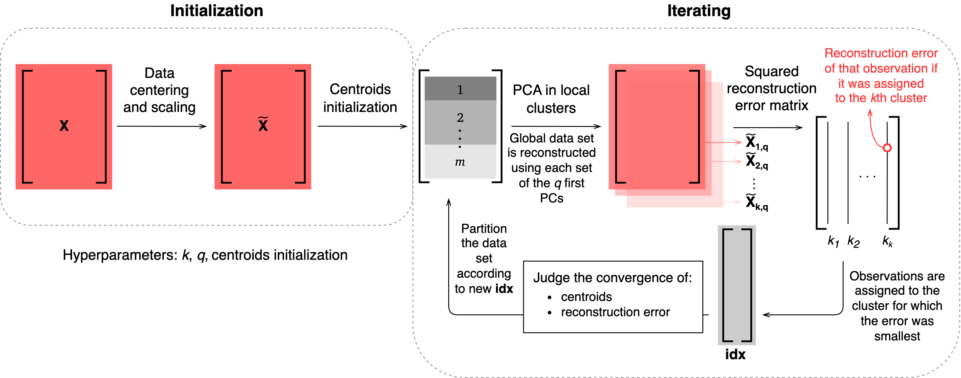

More information can be found in [ZdybalDAlessioA+23].

Note

The VQPCA algorithm centers the global data set \(\mathbf{X}\) by the mean value and scales it by the scaling specified with the scaling parameter. Data in local clusters is centered by the mean value but is not scaled.

Example:

from PCAfold import VQPCA
import numpy as np

# Generate dummy data set:
X = np.random.rand(400,10)

# Instantiate VQPCA class object:
vqpca = VQPCA(X,
              n_clusters=3,
              n_components=2,
              scaling='std',
              idx_init='random',
              max_iter=100,
              tolerance=1.0e-08,
              random_state=42,
              verbose=True)

# Access the VQPCA clustering solution:
idx = vqpca.idx

With verbose=True, the code above will print detailed information on each iteration:

| It.   | Rec. error      | Error conv.? | Cent. conv.? | Cluster 1  | Cluster 2  | Cluster 3  | Time [min]   |
| 1     | 10.20073505     | False        | False        | 165        | 58         | 177        | 0.00042      |
| 2     | 6.02108074      | False        | False        | 155        | 84         | 161        | 0.00073      |
| 3     | 5.79390739      | False        | False        | 148        | 97         | 155        | 0.0011       |
| 4     | 5.69141601      | False        | False        | 148        | 110        | 142        | 0.00134      |
| 5     | 5.63347972      | False        | False        | 148        | 117        | 135        | 0.00156      |
| 6     | 5.61523762      | False        | False        | 148        | 117        | 135        | 0.00175      |
| 7     | 5.61010989      | False        | False        | 147        | 117        | 136        | 0.00199      |
| 8     | 5.60402719      | False        | False        | 144        | 119        | 137        | 0.00224      |
| 9     | 5.59803052      | False        | False        | 144        | 121        | 135        | 0.00246      |
| 10    | 5.59072799      | False        | False        | 142        | 123        | 135        | 0.00268      |
| 11    | 5.5783608       | False        | False        | 139        | 123        | 138        | 0.00291      |
| 12    | 5.57368963      | False        | False        | 138        | 123        | 139        | 0.00316      |
| 13    | 5.56762599      | False        | False        | 140        | 122        | 138        | 0.0034       |
| 14    | 5.55839038      | False        | False        | 138        | 120        | 142        | 0.00368      |
| 15    | 5.55167405      | False        | False        | 137        | 120        | 143        | 0.00394      |
| 16    | 5.54661554      | False        | False        | 136        | 120        | 144        | 0.0042       |
| 17    | 5.5453694       | False        | True         | 136        | 120        | 144        | 0.00444      |
| 18    | 5.5453694       | True         | True         | 136        | 120        | 144        | 0.00444      |
Convergence reached in iteration: 18

Total time: 0.004471 minutes.
--------------------------------------------------------------------------------------------------------------

Parameters:

X – numpy.ndarray specifying the original data set, \(\mathbf{X}\). It should be of size (n_observations,n_variables).
n_clusters – int specifying the number of clusters to partition the data.
n_components – (optional) int specifying the number of retained principal components, \(q\). If set to 0 all PCs are retained. It should be a non-negative number.
scaling – str specifying the scaling methodology. It can be one of the following: 'none', '', 'auto', 'std', 'pareto', 'vast', 'range', '0to1', '-1to1', 'level', 'max', 'variance', 'median', 'poisson', 'vast_2', 'vast_3', 'vast_4'.
idx_init – (optional) str or numpy.ndarray specifying the method for centroids initialization. If str, it can be 'uniform' or 'random'. By default random intialization is performed. An arbitrary user-supplied initial idx for initializing the centroids can be passed using a numpy.ndarray. It should be of size (n_observations,) or (n_observations,1).
max_iter – (optional) the maximum number of iterations that the algorithm will loop through.
tolerance – (optional) float specifying the tolerance for the global mean squared reconstruction error and for the cluster centroids. This parameter is important for judging the convergence of the VQPCA algorithm. If set to None, the default value 1.0e-08 is used.
random_state – (optional) int specifying the random seed.
verbose – (optional) boolean for printing clustering details.

Attributes:

idx - vector of cluster classifications.
collected_idx - vector of cluster classifications from all iterations.
converged - boolean specifying whether the algorithm has converged.
A - local eigenvectors from the last iteration.
principal_components - local Principal Components from the last iteration.
reconstruction_errors_in_clusters - mean reconstruction errors in each cluster from the last iteration.

Subset Principal Component Analysis#

Class `SubsetPCA`#

class PCAfold.reduction.SubsetPCA(X, X_source=None, full_sequence=True, subset_indices=None, variable_names=None, scaling='std', n_components=2, use_eigendec=True, nocenter=False, verbose=False)#

Enables performing Principal Component Analysis (PCA) of a subset of the original data set, \(\mathbf{X}\).

Example:

from PCAfold import SubsetPCA
import numpy as np

# Generate dummy data set:
X = np.random.rand(100,10)

# Instantiate SubsetPCA class object:
subset_pca_X = SubsetPCA(X, full_sequence=True, scaling='std', n_components=2)

Parameters:

X – numpy.ndarray specifying the original data set, \(\mathbf{X}\). It should be of size (n_observations,n_variables).
X_source – (optional) numpy.ndarray specifying the source terms, \(\mathbf{S_X}\), corresponding to the state-space variables in \(\mathbf{X}\). This parameter is applicable to data sets representing reactive flows. More information can be found in [SP09].
full_sequence – (optional) bool specifying if a full sequence of subset PCAs should be performed. If set to True, it is assumed that variables in \(\mathbf{X}\) have been ordered according to some criterion. A sequence of subset PCAs will then be performed starting from the first n_components+1 variables and gradually adding the next variable in \(\mathbf{X}\). When full_sequence=True, parameter subset_indices will be ignored and the class attributes will be of type list of numpy.ndarray. Each element in those lists corresponds to one subset PCA in a sequence.
subset_indices – (optional) list specifying the indices of columns to be taken from the original data set to form a subset of a data set.
variable_names – (optional) list of str specifying the names of variables in \(\mathbf{X}\). It should have length n_variables and each element should correspond to a column in \(\mathbf{X}\).
scaling – (optional) str specifying the scaling methodology. It can be one of the following: 'none', '', 'auto', 'std', 'pareto', 'vast', 'range', '0to1', '-1to1', 'level', 'max', 'variance', 'median', 'poisson', 'vast_2', 'vast_3', 'vast_4'.
n_components – (optional) int specifying the number of retained principal components, \(q\). If set to 0 all PCs are retained. It should be a non-negative number.
use_eigendec –
(optional) bool specifying the method for obtaining eigenvalues and eigenvectors:
- use_eigendec=True uses eigendecomposition of the covariance matrix (from numpy.linalg.eigh)
- use_eigendec=False uses Singular Value Decomposition (SVD) (from scipy.linalg.svd)
nocenter – (optional) bool specifying whether the data original data set should be centered by mean.

Attributes:

S - (read only) numpy.ndarray or list of numpy.ndarray specifying the covariance matrix, \(\mathbf{S}\).
L - (read only) numpy.ndarray or list of numpy.ndarray specifying the vector of eigenvalues, \(\mathbf{L}\).
A - (read only) numpy.ndarray or list of numpy.ndarray specifying the matrix of eigenvectors, \(\mathbf{A}\).
principal_components - (read only) numpy.ndarray or list of numpy.ndarray specifying the principal components, \(\mathbf{Z}\).
PC_source_terms - (read only) numpy.ndarray or list of numpy.ndarray specifying the PC source terms, \(\mathbf{S_Z}\).
variable_sequence - (read only) list or list of list specifying the names of variables that were used in each subset PCA.

Sample Principal Component Analysis#

Class `SamplePCA`#

PCAfold.reduction.SamplePCA(X, idx_X_r, scaling, n_components, biasing_option, X_source=None)#

Enables performing Principal Component Analysis (PCA) on a sample, \(\mathbf{X_r}\), of the original data set, \(\mathbf{X}\), with one of the four implemented options. Reach out to the Biasing options section of the documentation for more information on the available options.

Example:

from PCAfold import DataSampler, SamplePCA
import numpy as np

# Generate dummy data set:
X = np.random.rand(100,10)

# Generate dummy sampling indices:
idx = np.zeros((100,)).astype(int)
idx[50:80] = 1
selection = DataSampler(idx)
(idx_X_r, _) = selection.number(20, test_selection_option=1)

# Instantiate SamplePCA class object:
sample_pca = SamplePCA(X,
                       idx_X_r,
                       scaling='auto',
                       n_components=2,
                       biasing_option=1,
                       X_source=None)

# Access the re-sampled PCs:
PCs_resampled = sample_pca.pc_scores

Parameters:

X – numpy.ndarray specifying the original data set, \(\mathbf{X}\). It should be of size (n_observations,n_variables).
idx_X_r – numpy.ndarray specifying the vector of indices that should be extracted from \(\mathbf{X}\) to form \(\mathbf{X_r}\). It should be of size (n_samples,) or (n_samples,1).
scaling – str specifying the scaling methodology. It can be one of the following: 'none', '', 'auto', 'std', 'pareto', 'vast', 'range', '0to1', '-1to1', 'level', 'max', 'variance', 'median', 'poisson', 'vast_2', 'vast_3', 'vast_4'.
n_components – int specifying the number of retained principal components, \(q\). If set to 0 all PCs are retained. It should be a non-negative number.
biasing_option – int specifying the biasing option. It can only attain values 1, 2, 3 or 4.
X_source – (optional) numpy.ndarray specifying the source terms, \(\mathbf{S_X}\), corresponding to the state-space variables in \(\mathbf{X}\). This parameter is applicable to data sets representing reactive flows. More information can be found in [SP09].

Attributes:

eigenvalues - (read only) numpy.ndarray specifying the biased eigenvalues, \(\mathbf{L_r}\).
eigenvectors - (read only) numpy.ndarray specifying the biased eigenvectors, \(\mathbf{A_r}\).
pc_scores - (read only) numpy.ndarray specifying the \(q\) first biased principal components, \(\mathbf{Z_r}\).
pc_sources - (read only) numpy.ndarray specifying the \(q\) first biased sources of principal components, \(\mathbf{S_{Z_r}}\). More information can be found in [SP09]. This parameter is only computed if X_source input parameter is specified.
C - (read only) numpy.ndarray specifying a vector of centers, \(\mathbf{C}\), that were used to preprocess the original full data set \(\mathbf{X}\).
D - (read only) numpy.ndarray specifying a vector of scales, \(\mathbf{D}\), that were used to preprocess the original full data set \(\mathbf{X}\).
C_r - (read only) numpy.ndarray specifying a vector of centers, \(\mathbf{C_r}\), that were used to preprocess the sampled data set \(\mathbf{X_r}\).
D_r - (read only) numpy.ndarray specifying a vector of scales, \(\mathbf{D_r}\), that were used to preprocess the sampled data set \(\mathbf{X_r}\).

Class `EquilibratedSamplePCA`#

PCAfold.reduction.EquilibratedSamplePCA(X, idx, scaling, n_components, biasing_option, X_source=None, n_iterations=10, stop_iter=0, random_seed=None, verbose=False)#

This implementation gradually (in n_iterations) equilibrates cluster populations heading towards population of the smallest cluster, in each cluster.

At each iteration it generates a reduced data set \(\mathbf{X_r}^{(i)}\) made up from new populations, performs PCA on that data set to find the \(i^{th}\) version of the eigenvectors. Depending on the option selected, it then does the projection of a data set (and optionally also its sources) onto the found eigenvectors.

Equilibration:

For the moment, there is only one way implemented for the equilibration. The smallest cluster is found and any larger \(j^{th}\) cluster’s observations are diminished at each iteration by:

\[\frac{N_j - N_s}{\verb|n_iterations|}\]

\(N_j\) is the number of observations in that \(j^{th}\) cluster and \(N_s\) is the number of observations in the smallest cluster. This is further illustrated on synthetic data set below:

../_images/cluster-equilibration-scheme.svg

Future implementation will include equilibration that slows down close to equilibrium.

Interpretation for the outputs:

This function returns 3D arrays eigenvectors, pc_scores and pc_sources that have the following structure:

../_images/cbpca-equilibrate-outputs.svg

Example:

from PCAfold import EquilibratedSamplePCA
import numpy as np

# Generate dummy data set:
X = np.random.rand(100,10)

# Generate dummy sampling indices:
idx = np.zeros((100,))
idx[50:80] = 1
idx = idx.astype(int)

# Instantiate EquilibratedSamplePCA class object:
equilibrated_pca = EquilibratedSamplePCA(X,
                                         idx,
                                         'auto',
                                         n_components=2,
                                         biasing_option=1,
                                         n_iterations=1,
                                         random_seed=100,
                                         verbose=True)

# Access the re-sampled PCs from the last (equilibrated) iteration:
PCs_resampled = equilibrated_pca.pc_scores[:,:,-1]

Parameters:

X – numpy.ndarray specifying the original data set, \(\mathbf{X}\). It should be of size (n_observations,n_variables).
idx – numpy.ndarray of cluster classifications. It should be of size (n_observations,) or (n_observations,1).
scaling – str specifying the scaling methodology. It can be one of the following: 'none', '', 'auto', 'std', 'pareto', 'vast', 'range', '0to1', '-1to1', 'level', 'max', 'variance', 'median', 'poisson', 'vast_2', 'vast_3', 'vast_4'.
X_source – numpy.ndarray specifying the source terms \(\mathbf{S_X}\) corresponding to the state-space variables in \(\mathbf{X}\). This parameter is applicable to data sets representing reactive flows. More information can be found in [SP09].
n_components – int specifying number of \(q\) first principal components that will be saved.
biasing_option – int specifying the biasing option. It can only attain values 1, 2, 3 or 4.
n_iterations – (optional) int specifying the number of iterations to loop over.
stop_iter – (optional) int specifying the index of iteration to stop.
random_seed – (optional) int specifying random seed for random sample selection.
verbose – (optional) bool for printing verbose details.

Returns:

eigenvalues - numpy.ndarray specifying the collected eigenvalues from each iteration.
eigenvectors - numpy.ndarray specifying the collected eigenvectors from each iteration. This is a 3D array of size (n_variables, n_components, n_iterations+1).
pc_scores - numpy.ndarray specifying the collected principal components from each iteration. This is a 3D array of size (n_observations, n_components, n_iterations+1).
pc_sources - numpy.ndarray specifying the collected sources of principal components from each iteration. This is a 3D array of size (n_observations, n_components, n_iterations+1).
idx_train - numpy.ndarray specifying the final training indices from the equilibrated iteration.
C_r - numpy.ndarray specifying a vector of final centers that were used to center the data set at the last (equilibration) iteration.
D_r - numpy.ndarray specifying a vector of final scales that were used to scale the data set at the last (equilibration) iteration.

PCAfold.reduction.analyze_centers_change(X, idx_X_r, variable_names=[], plot_variables=[], legend_label=[], figure_size=None, title=None, save_filename=None)#

Analyzes the change in normalized centers computed on the sampled subset of the original data set \(\mathbf{X_r}\) with respect to the full original data set \(\mathbf{X}\).

The original data set \(\mathbf{X}\) is first normalized so that each variable ranges from 0 to 1:

\[||\mathbf{X}|| = \frac{\mathbf{X} - min(\mathbf{X})}{max(\mathbf{X} - min(\mathbf{X}))}\]

This normalization is done so that centers can be compared across variables on one plot. Samples are then extracted from \(||\mathbf{X}||\), according to idx_X_r, to form \(||\mathbf{X_r}||\).

Normalized centers are computed as:

\[||\mathbf{C}|| = mean(||\mathbf{X}||)\]

\[||\mathbf{C_r}|| = mean(||\mathbf{X_r}||)\]

Percentage measuring the relative change in normalized centers is computed as:

\[p = \frac{||\mathbf{C_r}|| - ||\mathbf{C}||}{||\mathbf{C}||} \cdot 100\%\]

Example:

from PCAfold import analyze_centers_change, DataSampler
import numpy as np

# Generate dummy data set:
X = np.random.rand(100,10)

# Generate dummy sampling indices:
idx = np.zeros((100,)).astype(int)
idx[50:80] = 1
selection = DataSampler(idx)
(idx_X_r, _) = selection.number(20, test_selection_option=1)

# Analyze the change in normalized centers:
(normalized_C, normalized_C_r, center_movement_percentage, plt) = analyze_centers_change(X, idx_X_r)

Parameters:

X – numpy.ndarray specifying the original data set, \(\mathbf{X}\). It should be of size (n_observations,n_variables).
idx_X_r – vector of indices that should be extracted from \(\mathbf{X}\) to form \(\mathbf{X_r}\).
variable_names – (optional) list of str specifying variable names.
plot_variables – (optional) list of int specifying indices of variables to be plotted. By default, all variables are plotted.
legend_label – (optional) list of str specifying labels for the legend. First entry will refer to \(||\mathbf{C}||\) and second entry to \(||\mathbf{C_r}||\). If the list is empty, legend will not be plotted.
figure_size – (optional) tuple specifying figure size.
title – (optional) str specifying plot title. If set to None title will not be plotted.
save_filename – (optional) str specifying plot save location/filename. If set to None plot will not be saved. You can also set a desired file extension, for instance .pdf. If the file extension is not specified, the default is .png.

Returns:

normalized_C - normalized centers \(||\mathbf{C}||\).
normalized_C_r - normalized centers \(||\mathbf{C_r}||\).
center_movement_percentage - percentage \(p\) measuring the relative change in normalized centers.
plt - matplotlib.pyplot plot handle.

PCAfold.reduction.analyze_eigenvector_weights_change(eigenvectors, variable_names=[], plot_variables=[], normalize=False, zero_norm=False, legend_label=[], color_map='viridis', figure_size=None, title=None, save_filename=None)#

Analyzes the change of weights on an eigenvector obtained from a reduced data set as specified by the eigenvectors matrix. This matrix can contain many versions of eigenvectors, for instance coming from each iteration from the equilibrate_cluster_populations function.

If the number of versions is larger than two, the weights are plot on a color scale that marks each version. If there is a consistent trend, the coloring should form a clear trajectory.

In a special case, when there are only two versions within eigenvectors matrix, it is understood that the first version corresponds to the original data set and the last version to the equilibrated data set.

Note: This function plots absolute, (and optionally normalized) values of weights on each variable. Columns are normalized dividing by the maximum value. This is done in order to compare the movement of weights equally, with the highest, normalized one being equal to 1. You can additionally set the zero_norm=True in order to normalize weights such that they are between 0 and 1 (this is not done by default).

Example:

from PCAfold import equilibrate_cluster_populations, analyze_eigenvector_weights_change
import numpy as np

# Generate dummy data set:
X = np.random.rand(100,10)

# Generate dummy sampling indices:
idx = np.zeros((100,))
idx[50:80] = 1

# Run cluster equlibration:
(eigenvalues, eigenvectors_matrix, pc_scores_matrix, pc_sources_matrix, idx_train, C_r, D_r) = equilibrate_cluster_populations(X, idx, 'auto', n_components=2, biasing_option=1, n_iterations=1, random_seed=100, verbose=True)

# Analyze weights change on the first eigenvector:
plt = analyze_eigenvector_weights_change(eigenvectors_matrix[:,0,:])

# Analyze weights change on the second eigenvector:
plt = analyze_eigenvector_weights_change(eigenvectors_matrix[:,1,:])

Parameters:

eigenvectors –
matrix of concatenated eigenvectors coming from different data sets or from different iterations. It should be size (n_variables, n_versions). This parameter can be directly extracted from eigenvectors_matrix output from function equilibrate_cluster_populations. For instance if the first and second eigenvector should be plotted:
```
eigenvectors_1 = eigenvectors_matrix[:,0,:]
eigenvectors_2 = eigenvectors_matrix[:,1,:]
```
variable_names – (optional) list of str specifying variable names.
plot_variables – (optional) list of integers specifying indices of variables to be plotted. By default, all variables are plotted.
normalize – (optional) bool specifying whether weights should be normlized at all. If set to false, the absolute values are plotted.
zero_norm – (optional) bool specifying whether weights should be normalized between 0 and 1. By default they are not normalized to start at 0. Only has effect if normalize=True.
legend_label – (optional) list of str specifying labels for the legend. If the list is empty, legend will not be plotted.
color_map – (optional) str or matplotlib.colors.ListedColormap specifying the colormap to use as per matplotlib.cm. Default is 'viridis'.
figure_size – (optional) tuple specifying figure size.
title – (optional) str specifying plot title. If set to None title will not be plotted.
save_filename – (optional) str specifying plot save location/filename. If set to None plot will not be saved. You can also set a desired file extension, for instance .pdf. If the file extension is not specified, the default is .png.

Returns:

plt - matplotlib.pyplot plot handle.

PCAfold.reduction.analyze_eigenvalue_distribution(X, idx_X_r, scaling, biasing_option, legend_label=[], figure_size=None, title=None, save_filename=None)#

Analyzes the normalized eigenvalue distribution when PCA is performed on the original data set \(\mathbf{X}\) and on the sampled data set \(\mathbf{X_r}\).

Reach out to the Biasing options section of the documentation for more information on the available options.

Example:

from PCAfold import analyze_eigenvalue_distribution, DataSampler
import numpy as np

# Generate dummy data set:
X = np.random.rand(100,10)

# Generate dummy sampling indices:
idx = np.zeros((100,)).astype(int)
idx[50:80] = 1
selection = DataSampler(idx)
(idx_X_r, _) = selection.number(20, test_selection_option=1)

# Analyze the change in eigenvalue distribution:
plt = analyze_eigenvalue_distribution(X, idx_X_r, 'auto', biasing_option=1)

Parameters:

X – numpy.ndarray specifying the original data set, \(\mathbf{X}\). It should be of size (n_observations,n_variables).
idx_X_r – vector of indices that should be extracted from \(\mathbf{X}\) to form \(\mathbf{X_r}\).
scaling – str specifying the scaling methodology. It can be one of the following: 'none', '', 'auto', 'std', 'pareto', 'vast', 'range', '0to1', '-1to1', 'level', 'max', 'variance', 'median', 'poisson', 'vast_2', 'vast_3', 'vast_4'.
biasing_option – int specifying biasing option. Can only attain values 1, 2, 3 or 4.
legend_label – (optional) list of str specifying labels for the legend. First entry will refer to \(\mathbf{X}\) and second entry to \(\mathbf{X_r}\). If the list is empty, legend will not be plotted.
figure_size – (optional) tuple specifying figure size.
title – (optional) str specifying plot title. If set to None title will not be plotted.
save_filename – (optional) str specifying plot save location/filename. If set to None plot will not be saved. You can also set a desired file extension, for instance .pdf. If the file extension is not specified, the default is .png.

Returns:

plt - matplotlib.pyplot plot handle.

Biasing options#

This section explains the choice for biasing_option input parameter in some of the functions in this module. The general goal for PCA on sampled data sets is to bias PCA with some information about the sampled data set \(\mathbf{X_r}\). Biasing option parameter will control how PCA is performed on or informed by \(\mathbf{X_r}\) data set sampled from \(\mathbf{X}\).

It is assumed that centers and scales computed on \(\mathbf{X_r}\) are denoted \(\mathbf{C_r}\) and \(\mathbf{D_r}\) and centers and scales computed on \(\mathbf{X}\) are denoted \(\mathbf{C}\) and \(\mathbf{D}\). \(N\) is the number of observations in \(\mathbf{X}\).

Biasing option 1#

The steps of PCA in this option:

Step	Option 1
S1: Sampling	\(\mathbf{X} \xrightarrow{\text{sampling}} \mathbf{X_r}\)
S2: Centering and scaling	\(\mathbf{X_{cs, r}} = (\mathbf{X_r} - \mathbf{C_r}) \cdot \mathbf{D_r}^{-1}\) \(\mathbf{X_{cs}} = (\mathbf{X} - \mathbf{C}) \cdot \mathbf{D}^{-1}\)
S3: PCA: Eigenvectors	\(\frac{1}{N-1} \mathbf{X_{cs, r}}^{\mathbf{T}} \mathbf{X_{cs, r}} \xrightarrow{\text{eigendec.}} \mathbf{A_r}\)
S4: PCA: Transformation	\(\mathbf{Z_r} = \mathbf{X_{cs}} \mathbf{A_r}\)

These steps are presented graphically below:

Biasing option 2#

The steps of PCA in this option:

Step	Option 2
S1: Sampling	\(\mathbf{X_{cs}} \xrightarrow{\text{sampling}} \mathbf{X_r}\)
S2: Centering and scaling	\(\mathbf{X_r}\) is not further pre-processed \(\mathbf{X_{cs}} = (\mathbf{X} - \mathbf{C}) \cdot \mathbf{D}^{-1}\)
S3: PCA: Eigenvectors	\(\frac{1}{N-1} \mathbf{X_r}^{\mathbf{T}} \mathbf{X_r} \xrightarrow{\text{eigendec.}} \mathbf{A_r}\)
S4: PCA: Transformation	\(\mathbf{Z_r} = \mathbf{X_{cs}} \mathbf{A_r}\)

These steps are presented graphically below:

Biasing option 3#

The steps of PCA in this option:

Step	Option 3
S1: Sampling	\(\mathbf{X} \xrightarrow{\text{sampling}} \mathbf{X_r}\)
S2: Centering and scaling	\(\mathbf{X_{cs, r}} = (\mathbf{X_r} - \mathbf{C_r}) \cdot \mathbf{D_r}^{-1}\) \(\mathbf{X_{cs}} = (\mathbf{X} - \mathbf{C_r}) \cdot \mathbf{D_r}^{-1}\)
S3: PCA: Eigenvectors	\(\frac{1}{N-1} \mathbf{X_{cs, r}}^{\mathbf{T}} \mathbf{X_{cs, r}} \xrightarrow{\text{eigendec.}} \mathbf{A_r}\)
S4: PCA: Transformation	\(\mathbf{Z_r} = \mathbf{X_{cs}} \mathbf{A_r}\)

These steps are presented graphically below:

Biasing option 4#

The steps of PCA in this option:

Step	Option 4
S1: Sampling	\(\mathbf{X} \xrightarrow{\text{sampling}} \mathbf{X_r}\)
S2: Centering and scaling	\(\mathbf{X_{cs}} = (\mathbf{X} - \mathbf{C_r}) \cdot \mathbf{D_r}^{-1}\)
S3: PCA: Eigenvectors	\(\frac{1}{N-1} \mathbf{X_{cs}}^{\mathbf{T}} \mathbf{X_{cs}} \xrightarrow{\text{eigendec.}} \mathbf{A_r}\)
S4: PCA: Transformation	\(\mathbf{Z_r} = \mathbf{X_{cs}} \mathbf{A_r}\)

These steps are presented graphically below:

Plotting functions#

PCAfold.reduction.plot_2d_manifold(x, y, color=None, clean=False, x_label=None, y_label=None, xscale=None, yscale=None, colorbar_label=None, color_map='viridis', colorbar_range=None, norm=None, grid_on=True, s=None, figure_size=(7, 7), title=None, save_filename=None)#

Plots a two-dimensional manifold given two vectors defining the manifold.

Example:

from PCAfold import PCA, plot_2d_manifold
import numpy as np

# Generate dummy data set:
X = np.random.rand(100,10)

# Obtain 2-dimensional manifold from PCA:
pca_X = PCA(X)
principal_components = pca_X.transform(X)

# Plot the manifold:
plt = plot_2d_manifold(principal_components[:,0],
                       principal_components[:,1],
                       color=X[:,0],
                       clean=False,
                       x_label='PC-1',
                       y_label='PC-2',
                       xscale=None,
                       yscale='log',
                       colorbar_label='$X_1$',
                       colorbar_range=(0,1),
                       figure_size=(5,5),
                       title='2D manifold',
                       save_filename='2d-manifold.pdf')
plt.close()

Parameters:

x – numpy.ndarray specifying the variable on the \(x\)-axis. It should be of size (n_observations,) or (n_observations,1).
y – numpy.ndarray specifying the variable on the \(y\)-axis. It should be of size (n_observations,) or (n_observations,1).
color – (optional) vector or string specifying color for the manifold. If it is a vector, it has to have length consistent with the number of observations in x and y vectors. It should be of type numpy.ndarray and size (n_observations,) or (n_observations,1). It can also be set to a string specifying the color directly, for instance 'r' or '#006778'. If not specified, manifold will be plotted in black.
clean – (optional) bool specifying if a clean plot should be made. If set to True, nothing else but the data points is plotted.
x_label – (optional) str specifying \(x\)-axis label annotation. If set to None label will not be plotted.
y_label – (optional) str specifying \(y\)-axis label annotation. If set to None label will not be plotted.
xscale – (optional) str specifying the scale for the \(x\)-axis. If set to None, axis will be plotted in linear scale.
yscale – (optional) str specifying the scale for the \(y\)-axis. If set to None, axis will be plotted in linear scale.
colorbar_label – (optional) str specifying colorbar label annotation. If set to None, colorbar label will not be plotted.
color_map – (optional) str or matplotlib.colors.ListedColormap specifying the colormap to use as per matplotlib.cm. Default is 'viridis'.
norm – (optional) matplotlib.colors specifying the colormap normalization to use. Example can be matplotlib.colors.LogNorm().
colorbar_range – (optional) tuple specifying the lower and the upper bound for the colorbar range.
grid_on – bool specifying whether grid should be plotted.
s – (optional) int or float specifying the scatter point size.
figure_size – (optional) tuple specifying figure size.
title – (optional) str specifying plot title. If set to None title will not be plotted.
save_filename – (optional) str specifying plot save location/filename. If set to None plot will not be saved. You can also set a desired file extension, for instance .pdf. If the file extension is not specified, the default is .png.

Returns:

plt - matplotlib.pyplot plot handle.

PCAfold.reduction.plot_3d_manifold(x, y, z, color=None, elev=45, azim=-45, clean=False, x_label=None, y_label=None, z_label=None, colorbar_label=None, color_map='viridis', colorbar_range=None, s=None, figure_size=(7, 7), title=None, save_filename=None)#

Plots a three-dimensional manifold given three vectors defining the manifold.

Example:

from PCAfold import PCA, plot_3d_manifold
import numpy as np

# Generate dummy data set:
X = np.random.rand(100,10)

# Obtain 3-dimensional manifold from PCA:
pca_X = PCA(X)
PCs = pca_X.transform(X)

# Plot the manifold:
plt = plot_3d_manifold(PCs[:,0],
                       PCs[:,1],
                       PCs[:,2],
                       color=X[:,0],
                       elev=30,
                       azim=-60,
                       clean=False,
                       x_label='PC-1',
                       y_label='PC-2',
                       z_label='PC-3',
                       colorbar_label='$X_1$',
                       colorbar_range=(0,1),
                       figure_size=(15,7),
                       title='3D manifold',
                       save_filename='3d-manifold.png')
plt.close()

Parameters:

x – variable on the \(x\)-axis. It should be of type numpy.ndarray and size (n_observations,) or (n_observations,1).
y – variable on the \(y\)-axis. It should be of type numpy.ndarray and size (n_observations,) or (n_observations,1).
z – variable on the \(z\)-axis. It should be of type numpy.ndarray and size (n_observations,) or (n_observations,1).
color – (optional) vector or string specifying color for the manifold. If it is a vector, it has to have length consistent with the number of observations in x, y and z vectors. It should be of type numpy.ndarray and size (n_observations,) or (n_observations,1). It can also be set to a string specifying the color directly, for instance 'r' or '#006778'. If not specified, manifold will be plotted in black.
elev – (optional) elevation angle.
azim – (optional) azimuth angle.
clean – (optional) bool specifying if a clean plot should be made. If set to True, nothing else but the data points and the 3D axes is plotted.
x_label – (optional) str specifying \(x\)-axis label annotation. If set to None label will not be plotted.
y_label – (optional) str specifying \(y\)-axis label annotation. If set to None label will not be plotted.
z_label – (optional) str specifying \(z\)-axis label annotation. If set to None label will not be plotted.
colorbar_label – (optional) str specifying colorbar label annotation. If set to None, colorbar label will not be plotted.
color_map – (optional) str or matplotlib.colors.ListedColormap specifying the colormap to use as per matplotlib.cm. Default is 'viridis'.
colorbar_range – (optional) tuple specifying the lower and the upper bound for the colorbar range.
s – (optional) int or float specifying the scatter point size.
figure_size – (optional) tuple specifying figure size.
title – (optional) str specifying plot title. If set to None title will not be plotted.
save_filename – (optional) str specifying plot save location/filename. If set to None plot will not be saved. You can also set a desired file extension, for instance .pdf. If the file extension is not specified, the default is .png.

Returns:

plt - matplotlib.pyplot plot handle.

PCAfold.reduction.plot_2d_manifold_sequence(xy, color=None, x_label=None, y_label=None, cbar=False, nrows=1, colorbar_label=None, color_map='viridis', grid_on=True, figure_size=(7, 3), title=None, save_filename=None)#

Plots a sequence of two-dimensional manifolds given a list of two vectors defining the manifold.

Example:

from PCAfold import SubsetPCA, plot_2d_manifold_sequence
import numpy as np

# Generate dummy data set:
X = np.random.rand(100,5)

# Obtain two-dimensional manifolds from subset PCA:
subset_PCA = SubsetPCA(X)
principal_components = subset_PCA.principal_components

# Plot the manifold:
plt = plot_2d_manifold_sequence(principal_components,
                                color=X[:,0],
                                x_label='PC-1',
                                y_label='PC-2',
                                nrows=2,
                                colorbar_label='$X_1$',
                                figure_size=(7,3),
                                title=['First', 'Second', 'Third'],
                                save_filename='2d-manifold-sequence.pdf')
plt.close()

Parameters:

xy – list of numpy.ndarray specifying the manifolds (variables on the \(x\) and \(y\) -axis). Each element of the list should be of size (n_observations,2).
color – (optional) numpy.ndarray or str, or list of numpy.ndarray or str specifying colors for the manifolds. If it is a vector, it has to have length consistent with the number of observations in x and y vectors. Each numpy.ndarray should be of size (n_observations,) or (n_observations,1). It can also be set to a string specifying the color directly, for instance 'r' or '#006778'. If not specified, manifolds will be plotted in black.
x_label – (optional) str specifying \(x\)-axis label annotation. If set to None label will not be plotted.
y_label – (optional) str specifying \(y\)-axis label annotation. If set to None label will not be plotted.
cbar – (optional) bool specifying if the colorbar should be plotted.
nrows – (optional) int specifying in how many rows the manifold sequence should be plotted.
colorbar_label – (optional) str specifying colorbar label annotation. If set to None, colorbar label will not be plotted.
color_map – (optional) str or matplotlib.colors.ListedColormap specifying the colormap to use as per matplotlib.cm. Default is 'viridis'.
grid_on – bool specifying whether grid should be plotted.
figure_size – (optional) tuple specifying figure size.
title – (optional) list of str specifying title for each subplot. If set to None titles will not be plotted.
save_filename – (optional) str specifying plot save location/filename. If set to None plot will not be saved. You can also set a desired file extension, for instance .pdf. If the file extension is not specified, the default is .png.

Returns:

plt - matplotlib.pyplot plot handle.

PCAfold.reduction.plot_parity(variable, variable_rec, color=None, x_label=None, y_label=None, colorbar_label=None, color_map='viridis', grid_on=True, figure_size=(7, 7), title=None, save_filename=None)#

Plots a parity plot between a variable and its reconstruction.

Example:

from PCAfold import PCA, plot_parity
import numpy as np

# Generate dummy data set:
X = np.random.rand(100,10)

# Obtain PCA reconstruction of the data set:
pca_X = PCA(X, n_components=8)
principal_components = pca_X.transform(X)
X_rec = pca_X.reconstruct(principal_components)

# Parity plot for the reconstruction of the first variable:
plt = plot_parity(X[:,0],
                  X_rec[:,0],
                  color=X[:,0],
                  x_label='Observed $X_1$',
                  y_label='Reconstructed $X_1$',
                  colorbar_label='X_1',
                  color_map='inferno',
                  figure_size=(5,5),
                  title='Parity plot',
                  save_filename='parity-plot.pdf')
plt.close()

Parameters:

variable – vector specifying the original variable. It should be of type numpy.ndarray and size (n_observations,) or (n_observations,1).
variable_rec – vector specifying the reconstruction of the original variable. It should be of type numpy.ndarray and size (n_observations,) or (n_observations,1).
color – (optional) vector or string specifying color for the parity plot. If it is a vector, it has to have length consistent with the number of observations in x and y vectors. It should be of type numpy.ndarray and size (n_observations,) or (n_observations,1). It can also be set to a string specifying the color directly, for instance 'r' or '#006778'. If not specified, parity plot will be plotted in black.
x_label – (optional) str specifying \(x\)-axis label annotation. If set to None label will not be plotted.
y_label – (optional) str specifying \(y\)-axis label annotation. If set to None label will not be plotted.
colorbar_label – (optional) str specifying colorbar label annotation. If set to None, colorbar label will not be plotted.
color_map – (optional) str or matplotlib.colors.ListedColormap specifying the colormap to use as per matplotlib.cm. Default is 'viridis'.
grid_on – bool specifying whether grid should be plotted.
figure_size – (optional) tuple specifying figure size.
title – (optional) str specifying plot title. If set to None title will not be plotted.
save_filename – (optional) str specifying plot save location/filename. If set to None plot will not be saved. You can also set a desired file extension, for instance .pdf. If the file extension is not specified, the default is .png.

Returns:

plt - matplotlib.pyplot plot handle.

PCAfold.reduction.plot_mode(mode, mode_name=None, variable_names=None, plot_absolute=False, rotate_label=False, bar_color=None, ylim=None, highlight_weights=None, highlight_color=None, figure_size=None, title=None, save_filename=None)#

Plots weights on a generic mode.

Example:

from PCAfold import PCA, plot_mode
import numpy as np

# Generate dummy data set:
X = np.random.rand(100,3)

# Perform PCA and obtain eigenvectors:
pca_X = PCA(X, n_components=2)
eigenvectors = pca_X.A

# Plot second and third eigenvector:
plt = plot_mode(eigenvectors[:,0],
                mode_name='PC',
                variable_names=['$a_1$', '$a_2$', '$a_3$'],
                plot_absolute=True,
                rotate_label=True,
                bar_color=None,
                ylim=None,
                highlight_weights=[0,1],
                highlight_color=['red', 'blue'],
                figure_size=(5,3),
                title='PCA on X',
                save_filename='PCA-X.pdf')

plt.close()

Parameters:

mode – numpy.ndarray specifying the mode to plot. It should be of size (n_variables,) or (n_variables,1).
mode_name – str specifying the mode name.
variable_names – (optional) list of str specifying variable names.
plot_absolute – (optional) bool specifying whether absolute values of eigenvectors should be plotted.
rotate_label – (optional) bool specifying whether the labels on the x-axis should be rotated by 90 degrees. It is recommended to set it to True for data sets with many variables for viewing clarity.
bar_color – (optional) str specifying color of bars.
ylim – (optional) list specifying limits on the y-axis.
highlight_weights – (optional) list of int specifying which variables to highlight with a different color.
highlight_color – (optional) str or list of str specifying the color(s) for the highlighted variables. By default, variables are highlighted in red.
figure_size – (optional) tuple specifying figure size.
title – (optional) str specifying plot title. If set to None title will not be plotted.
save_filename – (optional) str specifying plot save location/filename. If set to None plot will not be saved. You can also set a desired file extension, for instance .pdf. If the file extension is not specified, the default is .png.

Returns:

plt - matplotlib.pyplot plot handle.

PCAfold.reduction.plot_eigenvectors(eigenvectors, eigenvectors_indices=[], variable_names=None, plot_absolute=False, rotate_label=False, bar_color=None, figure_size=None, title=None, save_filename=None)#

Plots weights on eigenvectors. It will generate as many plots as there are eigenvectors present in the eigenvectors matrix.

Example:

from PCAfold import PCA, plot_eigenvectors
import numpy as np

# Generate dummy data set:
X = np.random.rand(100,3)

# Perform PCA and obtain eigenvectors:
pca_X = PCA(X, n_components=2)
eigenvectors = pca_X.A

# Plot second and third eigenvector:
plts = plot_eigenvectors(eigenvectors[:,[1,2]],
                         eigenvectors_indices=[1,2],
                         variable_names=['$a_1$', '$a_2$', '$a_3$'],
                         plot_absolute=False,
                         rotate_label=True,
                         bar_color=None,
                         title='PCA on X',
                         save_filename='PCA-X.pdf')
plts[0].close()
plts[1].close()

Parameters:

eigenvectors – matrix of eigenvectors to plot. It can be supplied as an attribute of the PCA class: PCA.A.
eigenvectors_indices – list of int specifying indexing of eigenvectors inside eigenvectors supplied. If it is not supplied, it is assumed that eigenvectors are numbered \([0, 1, 2, \dots, n]\), where \(n\) is the number of eigenvectors provided.
variable_names – (optional) list of str specifying variable names.
plot_absolute – (optional) bool specifying whether absolute values of eigenvectors should be plotted.
rotate_label – (optional) bool specifying whether the labels on the x-axis should be rotated by 90 degrees. It is recommended to set it to True for data sets with many variables for viewing clarity.
bar_color – (optional) str specifying color of bars.
figure_size – (optional) tuple specifying figure size.
title – (optional) str specifying plot title. If set to None title will not be plotted.
save_filename – (optional) str specifying plot save location/filename. If set to None plot will not be saved. You can also set a desired file extension, for instance .pdf. If the file extension is not specified, the default is .png. Note that a prefix eigenvector-# will be added out front the filename, where # is the number of the currently plotted eigenvector.

Returns:

plot_handles - list of plot handles.

PCAfold.reduction.plot_eigenvectors_comparison(eigenvectors_tuple, legend_labels=[], variable_names=[], plot_absolute=False, rotate_label=False, ylim=None, color_map='coolwarm', figure_size=None, title=None, save_filename=None)#

Plots a comparison of weights on eigenvectors.

Example:

from PCAfold import PCA, plot_eigenvectors_comparison
import numpy as np

# Generate dummy data set:
X = np.random.rand(100,3)

# Perform PCA and obtain eigenvectors:
pca_X = PCA(X, n_components=2)
eigenvectors = pca_X.A

# Plot comparaison of first and second eigenvector:
plt = plot_eigenvectors_comparison((eigenvectors[:,0],
                                    eigenvectors[:,1]),
                                   legend_labels=['PC-1', 'PC-2'],
                                   variable_names=['$a_1$', '$a_2$', '$a_3$'],
                                   plot_absolute=False,
                                   color_map='coolwarm',
                                   title='PCA on X',
                                   save_filename='PCA-X.pdf')
plt.close()

Parameters:

eigenvectors_tuple – tuple specifying the eigenvectors to plot. Each eigenvector inside a tuple should be a 0D array. It can be supplied as an attribute of the PCA class, for instance: (PCA.A[:,0], PCA.A[:,1]).
legend_labels – list of str specifying labels for each element in the eigenvectors_tuple.
variable_names – (optional) list of str specifying variable names.
plot_absolute – bool specifying whether absolute values of eigenvectors should be plotted.
rotate_label – (optional) bool specifying whether the labels on the x-axis should be rotated by 90 degrees. It is recommended to set it to True for data sets with many variables for viewing clarity.
color_map – (optional) str or matplotlib.colors.ListedColormap specifying the colormap to use as per matplotlib.cm. Default is 'coolwarm'.
figure_size – (optional) tuple specifying figure size.
title – (optional) str specifying plot title. If set to None title will not be plotted.
save_filename – (optional) str specifying plot save location/filename. If set to None plot will not be saved. You can also set a desired file extension, for instance .pdf. If the file extension is not specified, the default is .png.

Returns:

plt - matplotlib.pyplot plot handle.

PCAfold.reduction.plot_eigenvalue_distribution(eigenvalues, normalized=False, figure_size=None, title=None, save_filename=None)#

Plots eigenvalue distribution.

Example:

from PCAfold import PCA, plot_eigenvalue_distribution
import numpy as np

# Generate dummy data set:
X = np.random.rand(100,5)

# Perform PCA and obtain eigenvalues:
pca_X = PCA(X)
eigenvalues = pca_X.L

# Plot eigenvalue distribution:
plt = plot_eigenvalue_distribution(eigenvalues,
                                   normalized=True,
                                   title='PCA on X',
                                   save_filename='PCA-X.pdf')
plt.close()

Parameters:

eigenvalues – a 0D vector of eigenvalues to plot. It can be supplied as an attribute of the PCA class: PCA.L.
normalized – (optional) bool specifying whether eigenvalues should be normalized to 1.
figure_size – (optional) tuple specifying figure size.
title – (optional) str specifying plot title. If set to None title will not be plotted.
save_filename – (optional) str specifying plot save location/filename. If set to None plot will not be saved. You can also set a desired file extension, for instance .pdf. If the file extension is not specified, the default is .png.

Returns:

plt - matplotlib.pyplot plot handle.

PCAfold.reduction.plot_eigenvalue_distribution_comparison(eigenvalues_tuple, legend_labels=[], normalized=False, color_map='coolwarm', figure_size=None, title=None, save_filename=None)#

Plots a comparison of eigenvalue distributions.

Example:

from PCAfold import PCA, plot_eigenvalue_distribution_comparison
import numpy as np

# Generate dummy data sets:
X = np.random.rand(100,10)
Y = np.random.rand(100,10)

# Perform PCA and obtain eigenvalues:
pca_X = PCA(X)
eigenvalues_X = pca_X.L
pca_Y = PCA(Y)
eigenvalues_Y = pca_Y.L

# Plot eigenvalue distribution comparison:
plt = plot_eigenvalue_distribution_comparison((eigenvalues_X, eigenvalues_Y),
                                              legend_labels=['PCA on X', 'PCA on Y'],
                                              normalized=True,
                                              title='PCA on X and Y',
                                              save_filename='PCA-X-Y.pdf')
plt.close()

Parameters:

eigenvalues_tuple – tuple specifying the eigenvalues to plot. Each vector of eigenvalues inside a tuple should be a 0D array. It can be supplied as an attribute of the PCA class, for instance: (PCA_1.L, PCA_2.L).
legend_labels – list of str specifying the labels for each element in the eigenvalues_tuple.
normalized – (optional) bool specifying whether eigenvalues should be normalized to 1.
color_map – (optional) str or matplotlib.colors.ListedColormap specifying the colormap to use as per matplotlib.cm. Default is 'coolwarm'.
figure_size – (optional) tuple specifying figure size.
title – (optional) str specifying plot title. If set to None title will not be plotted.
save_filename – (optional) str specifying plot save location/filename. If set to None plot will not be saved. You can also set a desired file extension, for instance .pdf. If the file extension is not specified, the default is .png.

Returns:

plt - matplotlib.pyplot plot handle.

PCAfold.reduction.plot_cumulative_variance(eigenvalues, n_components=0, figure_size=None, title=None, save_filename=None)#

Plots the eigenvalues as bars and their cumulative sum to visualize the percent variance in the data explained by each principal component individually and by each principal component cumulatively.

Example:

from PCAfold import PCA, plot_cumulative_variance
import numpy as np

# Generate dummy data set:
X = np.random.rand(100,5)

# Perform PCA and obtain eigenvalues:
pca_X = PCA(X)
eigenvalues = pca_X.L

# Plot the cumulative variance from eigenvalues:
plt = plot_cumulative_variance(eigenvalues,
                               n_components=0,
                               title='PCA on X',
                               save_filename='PCA-X.pdf')
plt.close()

Parameters:

eigenvalues – a 0D vector of eigenvalues to analyze. It can be supplied as an attribute of the PCA class: PCA.L.
n_components – (optional) how many principal components you want to visualize (default is all).
figure_size – (optional) tuple specifying figure size.
title – (optional) str specifying plot title. If set to None title will not be plotted.
save_filename – (optional) str specifying plot save location/filename. If set to None plot will not be saved. You can also set a desired file extension, for instance .pdf. If the file extension is not specified, the default is .png.

Returns:

plt - matplotlib.pyplot plot handle.

PCAfold.reduction.plot_heatmap(M, annotate=False, text_color='w', format_displayed='%.2f', x_ticks=None, y_ticks=None, color_map='viridis', cbar=False, colorbar_label=None, figure_size=(5, 5), title=None, save_filename=None)#

Plots a heatmap for any matrix \(\mathbf{M}\).

Example:

from PCAfold import PCA, plot_heatmap
import numpy as np

# Generate dummy data set:
X = np.random.rand(100,5)

# Perform PCA and obtain the covariance matrix:
pca_X = PCA(X)
covariance_matrix = pca_X.S

# Define ticks:
ticks = ['A', 'B', 'C', 'D', 'E']

# Plot a heatmap of the covariance matrix:
plt = plot_heatmap(covariance_matrix,
                   annotate=True,
                   text_color='w',
                   format_displayed='%.1f',
                   x_ticks=ticks,
                   y_ticks=ticks,
                   title='Covariance',
                   save_filename='covariance.pdf')
plt.close()

Parameters:

M – numpy.ndarray specifying the matrix \(\mathbf{M}\).
annotate – (optional) bool specifying whether numerical values of matrix elements should be plot on top of the heatmap.
text_color – (optional) str specifying the color of the annotation text.
format_displayed – (optional) str specifying the display format for the numerical entries inside the table. By default it is set to '%.2f'.
x_ticks – (optional) bool specifying whether ticks on the \(x\) -axis should be plotted or list specifying the ticks on the \(x\) -axis.
y_ticks – (optional) bool specifying whether ticks on the \(y\) -axis should be plotted or list specifying the ticks on the \(y\) -axis.
color_map – (optional) str or matplotlib.colors.ListedColormap specifying the colormap to use as per matplotlib.cm. Default is 'viridis'.
cbar – (optional) bool specifying whether colorbar should be plotted.
colorbar_label – (optional) str specifying colorbar label annotation. If set to None, colorbar label will not be plotted.
figure_size – (optional) tuple specifying figure size.
title – (optional) str specifying plot title. If set to None title will not be plotted.
save_filename – (optional) str specifying plot save location/filename. If set to None plot will not be saved. You can also set a desired file extension, for instance .pdf. If the file extension is not specified, the default is .png.

Returns:

plt - matplotlib.pyplot plot handle.

PCAfold.reduction.plot_heatmap_sequence(M, annotate=False, text_color='w', format_displayed='%.2f', x_ticks=None, y_ticks=None, color_map='viridis', cbar=False, colorbar_label=None, figure_size=(5, 5), title=None, save_filename=None)#

Plots a sequence of heatmaps for matrices \(\mathbf{M}\) stored in a list.

Example:

from PCAfold import PCA, plot_heatmap_sequence
import numpy as np

# Generate dummy data set:
X = np.random.rand(100,5)

# Perform PCA and obtain the covariance matrices:
pca_X_auto = PCA(X, scaling='auto')
pca_X_range = PCA(X, scaling='range')
pca_X_vast = PCA(X, scaling='vast')
covariance_matrices = [pca_X_auto.S, pca_X_range.S, pca_X_vast.S]
titles = ['Auto', 'Range', 'VAST']

# Plot a sequence of heatmaps of the covariance matrices:
plt = plot_heatmap_sequence(covariance_matrices,
                            annotate=True,
                            text_color='w',
                            format_displayed='%.1f',
                            color_map='viridis',
                            cbar=True,
                            title=titles,
                            figure_size=(12,3),
                            save_filename='covariance-matrices.pdf')
plt.close()

Parameters:

M – list of numpy.ndarray specifying the matrices \(\mathbf{M}\).
annotate – (optional) bool specifying whether numerical values of matrix elements should be plot on top of the heatmap.
text_color – (optional) str specifying the color of the annotation text.
format_displayed – (optional) str specifying the display format for the numerical entries inside the table. By default it is set to '%.2f'.
x_ticks – (optional) bool specifying whether ticks on the \(x\) -axis should be plotted or list of list specifying the ticks on the \(x\) -axis.
y_ticks – (optional) bool specifying whether ticks on the \(y\) -axis should be plotted or list of list specifying the ticks on the \(y\) -axis.
color_map – (optional) str or matplotlib.colors.ListedColormap specifying the colormap to use as per matplotlib.cm. Default is 'viridis'.
cbar – (optional) bool specifying whether colorbar should be plotted.
colorbar_label – (optional) str specifying colorbar label annotation. If set to None, colorbar label will not be plotted.
figure_size – (optional) tuple specifying figure size.
title – (optional) str specifying plot title. If set to None title will not be plotted.
save_filename – (optional) str specifying plot save location/filename. If set to None plot will not be saved. You can also set a desired file extension, for instance .pdf. If the file extension is not specified, the default is .png.

Returns:

plt - matplotlib.pyplot plot handle.

Module: reduction#

Principal Component Analysis#

Class PCA#

Local Principal Component Analysis#

Class LPCA#

Vector Quantization Principal Component Analysis#

Class VQPCA#

Subset Principal Component Analysis#

Class SubsetPCA#

Sample Principal Component Analysis#

Class SamplePCA#

Class EquilibratedSamplePCA#

Biasing options#

Biasing option 1#

Biasing option 2#

Biasing option 3#

Biasing option 4#

Plotting functions#

Class `PCA`#

Class `LPCA`#

Class `VQPCA`#

Class `SubsetPCA`#

Class `SamplePCA`#

Class `EquilibratedSamplePCA`#