Module: analysis

The analysis module contains functions for assessing the intrinsic dimensionality and quality of manifolds.

Note

The format for the user-supplied input data matrix \(\mathbf{X} \in \mathbb{R}^{N \times Q}\), common to all modules, is that \(N\) observations are stored in rows and \(Q\) variables are stored in columns. Since typically \(N \gg Q\), the initial dimensionality of the data set is determined by the number of variables, \(Q\).

\[\begin{split}\mathbf{X} = \begin{bmatrix} \vdots & \vdots & & \vdots \\ X_1 & X_2 & \dots & X_{Q} \\ \vdots & \vdots & & \vdots \\ \end{bmatrix}\end{split}\]

The general agreement throughout this documentation is that \(i\) will index observations and \(j\) will index variables.

The representation of the user-supplied data matrix in PCAfold is the input parameter X, which should be of type numpy.ndarray and of size (n_observations,n_variables).

---

Manifold assessment

This section includes functions for quantitative assessments of manifold dimensionality and for comparing manifold parameterizations according to scales of variation and uniqueness of dependent variable values as introduced in [AS21] and [ZdybalASP22].

PCAfold.analysis.compute_normalized_variance(indepvars, depvars, depvar_names, npts_bandwidth=25, min_bandwidth=None, max_bandwidth=None, bandwidth_values=None, scale_unit_box=True, n_threads=None, compute_sample_norm_var=False, compute_sample_norm_range=False)

Compute a normalized variance (and related quantities) for analyzing manifold dimensionality. The normalized variance is computed as

\[\mathcal{N}(\sigma) = \frac{\sum_{i=1}^n (y_i - \mathcal{K}(\hat{x}_i; \sigma))^2}{\sum_{i=1}^n (y_i - \bar{y} )^2}\]

where \(\bar{y}\) is the average quantity over the whole manifold and \(\mathcal{K}(\hat{x}_i; \sigma)\) is the weighted average quantity calculated using kernel regression with a Gaussian kernel of bandwidth \(\sigma\) centered around the \(i^{th}\) observation. \(n\) is the number of observations. \(\mathcal{N}(\sigma)\) is computed for each bandwidth in an array of bandwidth values. By default, the indepvars (\(x\)) are centered and scaled to reside inside a unit box (resulting in \(\hat{x}\)) so that the bandwidths have the same meaning in each dimension. Therefore, the bandwidth and its involved calculations are applied in the normalized independent variable space. This may be turned off by setting scale_unit_box to False. The bandwidth values may be specified directly through bandwidth_values or default values will be calculated as a logspace from min_bandwidth to max_bandwidth with npts_bandwidth number of values. If left unspecified, min_bandwidth and max_bandwidth will be calculated as the minimum and maximum nonzero distance between points, respectively.

More information can be found in [AS21].

Example:

from PCAfold import PCA, compute_normalized_variance
import numpy as np

# Generate dummy data set:
X = np.random.rand(100,5)

# Perform PCA to obtain the low-dimensional manifold:
pca_X = PCA(X, n_components=2)
principal_components = pca_X.transform(X)

# Specify the bandwidth values:
bandwidth_values = np.logspace(-3, 1, 20)

# Compute normalized variance quantities:
variance_data = compute_normalized_variance(principal_components,
                                            X,
                                            depvar_names=['A', 'B', 'C', 'D', 'E'],
                                            bandwidth_values=bandwidth_values,
                                            scale_unit_box=True)

# Access bandwidth values:
variance_data.bandwidth_values

# Access normalized variance values:
variance_data.normalized_variance

# Access normalized variance values for a specific variable:
variance_data.normalized_variance['B']

Parameters:

• indepvars – numpy.ndarray specifying the independent variable values. It should be of size (n_observations,n_independent_variables).

• depvars – numpy.ndarray specifying the dependent variable values. It should be of size (n_observations,n_dependent_variables).

• depvar_names – list of str corresponding to the names of the dependent variables (for saving values in a dictionary)

• npts_bandwidth – (optional, default 25) number of points to build a logspace of bandwidth values

• min_bandwidth – (optional, default to minimum nonzero interpoint distance) minimum bandwidth

• max_bandwidth – (optional, default to estimated maximum interpoint distance) maximum bandwidth

• bandwidth_values – (optional) array of bandwidth values, i.e. filter widths for a Gaussian filter, to loop over

• scale_unit_box – (optional, default True) center/scale the independent variables between [0,1] for computing a normalized variance so the bandwidth values have the same meaning in each dimension

• n_threads – (optional, default None) number of threads to run this computation. If None, default behavior of multiprocessing.Pool is used, which is to use all available cores on the current system.

• compute_sample_norm_var – (optional, default False) bool specifying if sample normalized variance should be computed.

• compute_sample_norm_range – (optional, default False) bool specifying if sample normalized range should be computed.

Returns:

• variance_data - an object of the VarianceData class.

PCAfold.analysis.compute_normalized_range(indepvars, labels, npts_bandwidth=25, min_bandwidth=None, max_bandwidth=None, bandwidth_values=None, scale_unit_box=True, activation_function='step', multiplier=3)

Computes a normalized range for analyzing manifold quality for categorical data. This function is an alternate version of the normalized variance (more information can be found in [AS21]) that is more suited to dealing with categorical data. We assume that class labels are used as the categorical dependent variable (as opposed to continuous dependent variable). For categorical data, the exact class labels may not carry any meaning, thus we are only interested in the fact that two different classes overlap each other. As an illustrative example, the same 2D manifold will be assessed as having the same quality for the two cases depicted in the figure below:

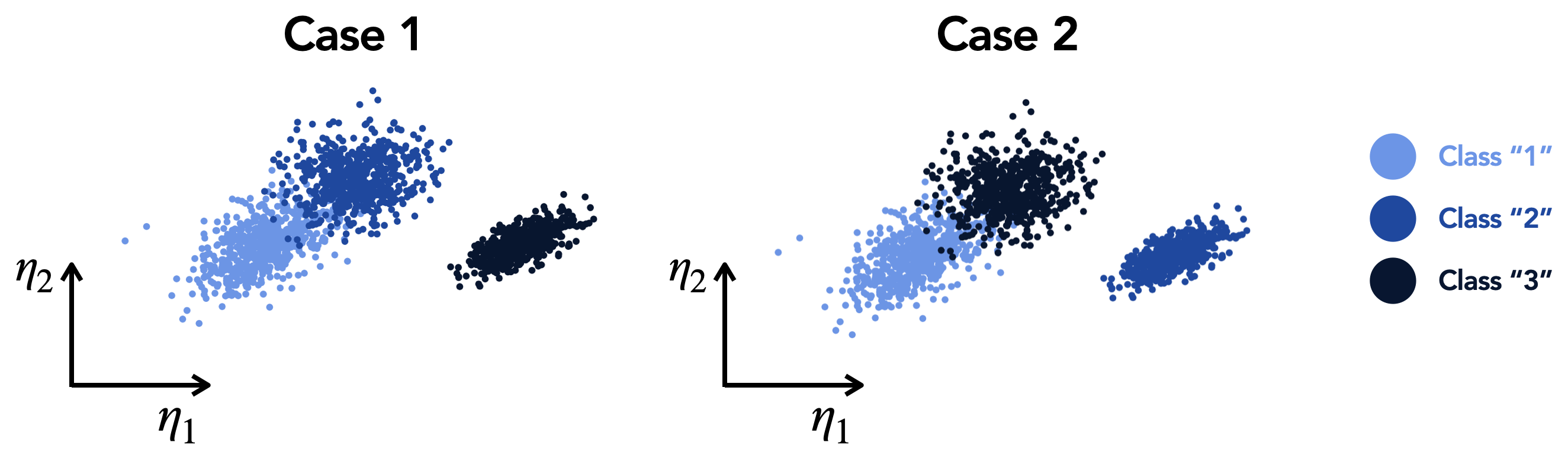
In Case 1, class “1” overlaps class “2” and in Case 2, class “1” overlaps class “3”. The normalized range will detect the fact that two different classes overlap each other, but it will neglect the fact which class labels those two classes have. In contrast, the normalized variance computed as per compute_normalized_variance will penalize overlap between classes “1” and “3” more than between classes “1” and “2”, simply because the difference between integers 1 and 3 is larger than between integers 1 and 2. The definition of the normalized range available in the present function corrects for that by passing each difference between class labels through an activation function, \(\mathcal{F}\), that returns 0 if two observations belong to the same class and a number larger than 0.0 but at most equal to 1.0 if two observations belong to two different classes.

The normalized range is computed as

\[\mathcal{N}(\sigma) = \frac{\sum_{i=1}^n \mathcal{F}((\Delta y_i|_{\sigma})^2)}{n}\]

where \(\Delta y_i|_{\sigma}\) is the range in the class labels (\(\min y_i - \max y_i\)) in the vicinity \(\sigma\) of the \(i\) th point, and \(\mathcal{F}\) is an activation function. \(n\) is the total number of observations (data points). \(\mathcal{N}(\sigma)\) is computed for each bandwidth in an array of bandwidth values.

Note

The numerator in the normalized range is at most equal to \(n\), thus we “normalize” the numerator by dividing by \(n\) in the denominator. This makes the normalized range bounded between 0.0 and 1.0.

Two activation functions are available:

• If activation_function is set to 'step' we use the following activation:

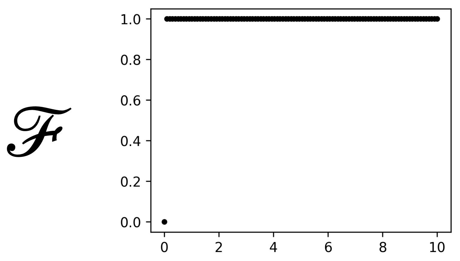\[\begin{split}\mathcal{F}(x) = \begin{cases} 0 &\text{if x = 0} \\ 1 &\text{if x > 0} \end{cases}\end{split}\]

• If activation_function is set to 'arctan' we use the following activation:

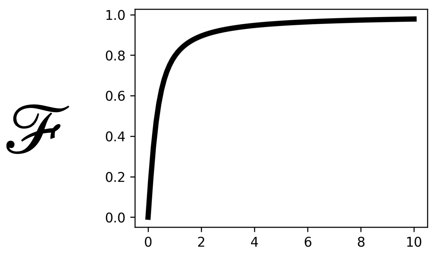\[\mathcal{F}(x) = \frac{\arctan(mx)}{\pi /2}\]

In the latter case, you can control how steep is the activation function using the multiplier parameter, \(m\).

By default, the indepvars (\(x\)) are centered and scaled to reside inside a unit box (resulting in \(\hat{x}\)) so that the bandwidths have the same meaning in each dimension. Therefore, the bandwidth and its involved calculations are applied in the normalized independent variable space. This may be turned off by setting scale_unit_box to False. The bandwidth values may be specified directly through bandwidth_values or default values will be calculated as a logspace from min_bandwidth to max_bandwidth with npts_bandwidth number of values. If left unspecified, min_bandwidth and max_bandwidth will be calculated as the minimum and maximum nonzero distance between points, respectively.

Example:

from PCAfold import PCA, compute_normalized_range
import numpy as np

# Generate dummy data set:
X = np.random.rand(100,5)

# Perform PCA to obtain the low-dimensional manifold:
pca_X = PCA(X, n_components=2)
principal_components = pca_X.transform(X)

# Generate dummy class labels:
idx = np.ones((100,))
idx[60:70] = 2
idx[71::] = 3

# Specify the bandwidth values:
bandwidth_values = np.logspace(-5, 1, 50)

# Compute normalized range:
variance_data = compute_normalized_range(principal_components,
                                         idx,
                                         bandwidth_values=bandwidth_values,
                                         scale_unit_box=True,
                                         activation_function='step')

Parameters:

• indepvars – numpy.ndarray specifying the independent variable values. It should be of size (n_observations,n_independent_variables).

• labels – numpy.ndarray specifying the dependent variable values (class labels). It should be of size (n_observations,) or (n_observations,1).

• npts_bandwidth – (optional) int specifying the number of points to build a logspace of bandwidth values.

• min_bandwidth – (optional) float specifying the minimum bandwidth.

• max_bandwidth – (optional) float specifying the maximum bandwidth

• bandwidth_values – (optional) numpy.ndarray specifying the array of bandwidth values, i.e., filter widths for a Gaussian filter, to loop over.

• scale_unit_box – (optional) bool specifying center/scale the independent variables between [0,1] for computing a normalized variance so the bandwidth values have the same meaning in each dimension.

• activation_function – (optional) str specifying the activation function. It should be 'step' or 'arctan'. If set to 'arctan', you may also control the steepness of the activation function with the multiplier parameter.

• multiplier – (optional) int or float specifying the multiplier, \(m\), to control the steepneess of the 'arctan' activation function. It is only used if activation_function is set to 'arctan'.

Returns:

• variance_data - an object of the VarianceData class.

PCAfold.analysis.normalized_variance_derivative(variance_data)

Compute a scaled normalized variance derivative on a logarithmic scale, \(\hat{\mathcal{D}}(\sigma)\), from

\[\mathcal{D}(\sigma) = \frac{\mathrm{d}\mathcal{N}(\sigma)}{\mathrm{d}\log_{10}(\sigma)} + \lim_{\sigma \to 0} \mathcal{N}(\sigma)\]

and

\[\hat{\mathcal{D}}(\sigma) = \frac{\mathcal{D}(\sigma)}{\max(\mathcal{D}(\sigma))}\]

This value relays how fast the variance is changing as the bandwidth changes and captures non-uniqueness from nonzero values of \(\lim_{\sigma \to 0} \mathcal{N}(\sigma)\). The derivative is approximated with central finite differencing and the limit is approximated by \(\mathcal{N}(\sigma=10^{-16})\) using the normalized_variance_limit attribute of the VarianceData object.

More information can be found in [AS21].

Example:

from PCAfold import PCA, compute_normalized_variance, normalized_variance_derivative
import numpy as np

# Generate dummy data set:
X = np.random.rand(100,5)

# Perform PCA to obtain the low-dimensional manifold:
pca_X = PCA(X, n_components=2)
principal_components = pca_X.transform(X)

# Specify the bandwidth values:
bandwidth_values = np.logspace(-3, 1, 20)

# Compute normalized variance quantities:
variance_data = compute_normalized_variance(principal_components,
                                            X,
                                            depvar_names=['A', 'B', 'C', 'D', 'E'],
                                            bandwidth_values=bandwidth_values,
                                            scale_unit_box=True)

# Compute normalized variance derivative:
(derivative, bandwidth_values, max_derivative) = normalized_variance_derivative(variance_data)

# Access normalized variance derivative values for a specific variable:
derivative['B']

Parameters:

variance_data – a VarianceData class returned from compute_normalized_variance

Returns:

• derivative_dict - a dictionary of \(\hat{\mathcal{D}}(\sigma)\) for each variable in the provided VarianceData object

• x - the \(\sigma\) values where \(\hat{\mathcal{D}}(\sigma)\) was computed

• max_derivatives_dicts - a dictionary of \(\max(\mathcal{D}(\sigma))\) values for each variable in the provided VarianceData object.

PCAfold.analysis.cost_function_normalized_variance_derivative(variance_data, penalty_function=None, power=1, vertical_shift=1, norm=None, integrate_to_peak=False, rightmost_peak_shift=None)

Defines a cost function for manifold topology assessment based on the areas, or weighted (penalized) areas, under the normalized variance derivatives curves, \(\hat{\mathcal{D}}(\sigma)\), for the selected \(n_{dep}\) dependent variables.

More information on the theory and application of the cost function can be found in [ZdybalASP22].

An individual area, \(A_i\), for the \(i^{th}\) dependent variable, is computed by directly integrating the function \(\hat{\mathcal{D}}_i(\sigma)`\) in the \(\log_{10}\) space of bandwidths \(\sigma\). Integration is performed using the composite trapezoid rule.

When integrate_to_peak=False, the bounds of integration go from the minimum bandwidth, \(\sigma_{min, i}\), to the maximum bandwidth, \(\sigma_{max, i}\):

\[A_i = \int_{\sigma_{min, i}}^{\sigma_{max, i}} \hat{\mathcal{D}}_i(\sigma) d \log_{10} \sigma\]

When integrate_to_peak=True, the bounds of integration go from the minimum bandwidth, \(\sigma_{min, i}\), to the bandwidth for which the rightmost peak happens in \(\hat{\mathcal{D}}_i(\sigma)`\), \(\sigma_{peak, i}\):

\[A_i = \int_{\sigma_{min, i}}^{\sigma_{peak, i}} \hat{\mathcal{D}}_i(\sigma) d \log_{10} \sigma\]

In addition, each individual area, \(A_i\), can be weighted. The following weighting options are available:

• If penalty_function='peak', \(A_i\) is weighted by the inverse of the rightmost peak location:

\[A_i = \frac{1}{\sigma_{peak, i}} \cdot \int \hat{\mathcal{D}}_i(\sigma) d(\log_{10} \sigma)\]

This creates a constant penalty:

• If penalty_function='sigma', \(A_i\) is weighted continuously by the bandwidth:

\[A_i = \int \frac{1}{\sigma^r} \cdot \hat{\mathcal{D}}_i(\sigma) d(\log_{10} \sigma)\]

where \(r\) is a hyper-parameter that can be controlled by the user. This type of weighting strongly penalizes the area happening at lower bandwidth values.

For instance, when \(r=0.2\):

When \(r=1\) (with the penalty corresponding to \(r=0.2\) plotted in gray in the background):

• If penalty_function='log-sigma-over-peak', \(A_i\) is weighted continuously by the \(\log_{10}\) -transformed bandwidth and takes into account information about the rightmost peak location.

\[A_i = \int \Big( \big| \log_{10} \Big( \frac{\sigma}{\sigma_{peak, i}} \Big) \big|^r + b \cdot \frac{\log_{10} \sigma_{max, i} - \log_{10} \sigma_{min, i}}{\log_{10} \sigma_{peak, i} - \log_{10} \sigma_{min, i}} \Big) \cdot \hat{\mathcal{D}}_i(\sigma) d(\log_{10} \sigma)\]

This type of weighting creates a more gentle penalty for the area happening further from the rightmost peak location. By increasing \(b\), the user can increase the amount of penalty applied to smaller feature sizes over larger ones. By increasing \(r\), the user can penalize non-uniqueness more strongly.

For instance, when \(r=1\):

When \(r=2\) (with the penalty corresponding to \(r=1\) plotted in gray in the background):

If norm=None, a list of costs for all dependent variables is returned. Otherwise, the final cost, \(\mathcal{L}\), can be computed from all \(A_i\) in a few ways, where \(n_{dep}\) is the number of dependent variables stored in the variance_data object:

• If norm='cumulative', \(\mathcal{L} = \sum_{i = 1}^{n_{dep}} A_i\).

• If norm='average', \(\mathcal{L} = \frac{1}{n_{dep}} \sum_{i = 1}^{n_{dep}} A_i\).

• If norm='L2', \(\mathcal{L} = \sqrt{\sum_{i = 1}^{n_{dep}} A_i^2}\).

• If norm='normalized-L2', \(\mathcal{L} = \frac{1}{n_{dep}} \sqrt{\sum_{i = 1}^{n_{dep}} A_i^2}\).

• If norm='max', \(\mathcal{L} = \text{max} (A_i)\).

• If norm='min', \(\mathcal{L} = \text{min} (A_i)\).

• If norm='median', \(\mathcal{L} = \text{median} (A_i)\).

Example:

from PCAfold import PCA, compute_normalized_variance, cost_function_normalized_variance_derivative
import numpy as np

# Generate dummy data set:
X = np.random.rand(100,10)

# Specify variables names
variable_names = ['X_' + str(i) for i in range(0,10)]

# Perform PCA to obtain the low-dimensional manifold:
pca_X = PCA(X, n_components=2)
principal_components = pca_X.transform(X)

# Specify the bandwidth values:
bandwidth_values = np.logspace(-4, 2, 50)

# Compute normalized variance quantities:
variance_data = compute_normalized_variance(principal_components,
                                            X,
                                            depvar_names=variable_names,
                                            bandwidth_values=bandwidth_values)

# Compute the cost for the current manifold:
cost = cost_function_normalized_variance_derivative(variance_data,
                                                    penalty_function='sigma',
                                                    power=0.5,
                                                    vertical_shift=1,
                                                    norm='max',
                                                    integrate_to_peak=True)

Parameters:

• variance_data – an object of VarianceData class.

• penalty_function – (optional) str specifying the weighting (penalty) applied to each area. Set penalty_function='peak' to weight each area by the rightmost peak location, \(\sigma_{peak, i}\), for the \(i^{th}\) dependent variable. Set penalty_function='sigma' to weight each area continuously by the bandwidth. Set penalty_function='log-sigma' to weight each area continuously by the \(\log_{10}\) -transformed bandwidth. Set penalty_function='log-sigma-over-peak' to weight each area continuously by the \(\log_{10}\) -transformed bandwidth, normalized by the right most peak location, \(\sigma_{peak, i}\). If penalty_function=None, the area is not weighted.

• power – (optional) float or int specifying the power, \(r\). It can be used to control how much penalty should be applied to variance happening at the smallest length scales.

• vertical_shift – (optional) float or int specifying the vertical shift multiplier, \(b\). It can be used to control how much penalty should be applied to feature sizes.

• norm – (optional) str specifying the norm to apply for all areas \(A_i\). norm='cumulative' uses the \(L_{1}\) norm, norm='average' uses an arithmetic average, norm='L2' uses the \(L_{2}\) norm, norm='normalized-L2' uses the \(L_{2}\) norm divided by the number of target variables, norm='max' uses the \(L_{\infty}\) norm, norm='min' uses a minimum area, and norm='median' uses a median area. If norm=None, a list of individual costs for all depedent variables is returned.

• integrate_to_peak – (optional) bool specifying whether an individual area for the \(i^{th}\) dependent variable should be computed only up the the rightmost peak location.

• rightmost_peak_shift – (optional) float or int specifying the percentage, \(p\), of shift in the rightmost peak location. If set to a number between 0 and 100, a quantity \(p/100 (\sigma_{max} - \sigma_{peak, i})\) is added to the rightmost peak location. It can be used to move the rightmost peak location further right, for instance if there is a blending of scales in the \(\hat{\mathcal{D}}(\sigma)\) profile.

Returns:

• cost - float specifying the normalized cost, \(\mathcal{L}\), or, if norm=None, a list of costs, \(A_i\), for each dependent variable.

PCAfold.analysis.find_local_maxima(dependent_values, independent_values, logscaling=True, threshold=0.01, show_plot=False)

Finds and returns locations and values of local maxima in a dependent variable given a set of observations. The functional form of the dependent variable is approximated with a cubic spline for smoother approximations to local maxima.

Parameters:

• dependent_values – observations of a single dependent variable such as \(\hat{\mathcal{D}}\) from normalized_variance_derivative (for a single variable).

• independent_values – observations of a single independent variable such as \(\sigma\) returned by normalized_variance_derivative

• logscaling – (optional, default True) this logarithmically scales independent_values before finding local maxima. This is needed for scaling \(\sigma\) appropriately before finding peaks in \(\hat{\mathcal{D}}\).

• threshold – (optional, default \(10^{-2}\)) local maxima found below this threshold will be ignored.

• show_plot – (optional, default False) when True, a plot of the dependent_values over independent_values (logarithmically scaled if logscaling is True) with the local maxima highlighted will be shown.

Returns:

• the locations of local maxima in dependent_values

• the local maxima values

PCAfold.analysis.random_sampling_normalized_variance(sampling_percentages, indepvars, depvars, depvar_names, n_sample_iterations=1, verbose=True, npts_bandwidth=25, min_bandwidth=None, max_bandwidth=None, bandwidth_values=None, scale_unit_box=True, n_threads=None)

Compute the normalized variance derivatives \(\hat{\mathcal{D}}(\sigma)\) for random samples of the provided data specified using sampling_percentages. These will be averaged over n_sample_iterations iterations. Analyzing the shift in peaks of \(\hat{\mathcal{D}}(\sigma)\) due to sampling can distinguish between characteristic features and non-uniqueness due to a transformation/reduction of manifold coordinates. True features should not show significant sensitivity to sampling while non-uniqueness/folds in the manifold will.

More information can be found in [AS21].

Parameters:

• sampling_percentages – list or 1D array of fractions (between 0 and 1) of the provided data to sample for computing the normalized variance

• indepvars – independent variable values (size: n_observations x n_independent variables)

• depvars – dependent variable values (size: n_observations x n_dependent variables)

• depvar_names – list of strings corresponding to the names of the dependent variables (for saving values in a dictionary)

• n_sample_iterations – (optional, default 1) how many iterations for each sampling_percentages to average the normalized variance derivative over

• verbose – (optional, default True) when True, progress statements are printed

• npts_bandwidth – (optional, default 25) number of points to build a logspace of bandwidth values

• min_bandwidth – (optional, default to minimum nonzero interpoint distance) minimum bandwidth

• max_bandwidth – (optional, default to estimated maximum interpoint distance) maximum bandwidth

• bandwidth_values – (optional) array of bandwidth values, i.e. filter widths for a Gaussian filter, to loop over

• scale_unit_box – (optional, default True) center/scale the independent variables between [0,1] for computing a normalized variance so the bandwidth values have the same meaning in each dimension

• n_threads – (optional, default None) number of threads to run this computation. If None, default behavior of multiprocessing.Pool is used, which is to use all available cores on the current system.

Returns:

• a dictionary of the normalized variance derivative (\(\hat{\mathcal{D}}(\sigma)\)) for each sampling percentage in sampling_percentages averaged over n_sample_iterations iterations

• the \(\sigma\) values used for computing \(\hat{\mathcal{D}}(\sigma)\)

• a dictionary of the VarianceData objects for each sampling percentage and iteration in sampling_percentages and n_sample_iterations

PCAfold.analysis.feature_size_map(variance_data, variable_name, cutoff=1, starting_bandwidth_idx='peak', use_variance=False, verbose=False)

Computes a map of local feature sizes on a manifold.

This technique has been introduced in [ZdybalAPS23].

Example:

from PCAfold import PCA, compute_normalized_variance, feature_size_map
import numpy as np

# Generate dummy data set:
X = np.random.rand(100,10)

# Specify variables names
variable_names = ['X_' + str(i) for i in range(0,10)]

# Perform PCA to obtain the low-dimensional manifold:
pca_X = PCA(X, n_components=2)
principal_components = pca_X.transform(X)

# Specify the bandwidth values:
bandwidth_values = np.logspace(-4, 2, 50)

# Compute normalized variance quantities:
variance_data = compute_normalized_variance(principal_components,
                                            X,
                                            depvar_names=variable_names,
                                            bandwidth_values=bandwidth_values,
                                            compute_sample_norm_var=True)

# Compute the feature size map:
feature_size_map = feature_size_map(variance_data,
                                    variable_name='X_1',
                                    cutoff=1,
                                    starting_bandwidth_idx='peak',
                                    use_variance=True,
                                    verbose=True)

Parameters:

• variance_data – an object of VarianceData class.

• variable_name – str specifying the name of the dependent variable for which the feature size map should be computed. It should be as per name specified when computing variance_data.

• cutoff – (optional) float or int specifying the cutoff percentage, \(p\). It should be a number between 0 and 100.

• starting_bandwidth_idx – (optional) int or str specifying the index of the starting bandwidth to compute the local feature sizes from. Local feature sizes computed will never be smaller than the starting bandwidth. If set to 'peak', the starting bandwidth will be automatically calculated as the rightmost peak, \(\sigma_{peak}\).

• use_variance – (optional) bool specifying whether sample normalized variance (use_variance=True) or sample normalized range (use_variance=False) should be used to compute the feature size map. When use_variance=True, the analysis.compute_normalized_variance() should be computed with the flag compute_sample_norm_var=True so that sample normalized variance is available. When use_variance=False, the analysis.compute_normalized_variance() should be computed with the flag compute_sample_norm_range=True so that sample normalized range is available.

• verbose – (optional) bool for printing verbose details.

Returns:

• feature_size_map - numpy.ndarray specifying the local feature sizes on a manifold, \(\mathbf{B}\). It has size (n_observations,).

PCAfold.analysis.feature_size_map_smooth(indepvars, feature_size_map, method='median', n_neighbors=10)

Smooths out a map of local feature sizes on a manifold.

Note

This function requires the scikit-learn module. You can install it through:

pip install scikit-learn

Example:

from PCAfold import PCA, compute_normalized_variance, feature_size_map, smooth_feature_size_map
import numpy as np

# Generate dummy data set:
X = np.random.rand(100,10)

# Specify variables names
variable_names = ['X_' + str(i) for i in range(0,10)]

# Perform PCA to obtain the low-dimensional manifold:
pca_X = PCA(X, n_components=2)
principal_components = pca_X.transform(X)

# Specify the bandwidth values:
bandwidth_values = np.logspace(-4, 2, 50)

# Compute normalized variance quantities:
variance_data = compute_normalized_variance(principal_components,
                                            X,
                                            depvar_names=variable_names,
                                            bandwidth_values=bandwidth_values)

# Compute the feature size map:
feature_size_map = feature_size_map(variance_data,
                                    variable_name='X_1',
                                    cutoff=1,
                                    starting_bandwidth_idx='peak',
                                    verbose=True)

# Smooth out the feature size map:
updated_feature_size_map = feature_size_map_smooth(principal_components,
                                                   feature_size_map,
                                                   method='median',
                                                   n_neighbors=4)

Parameters:

• indepvars – numpy.ndarray specifying the independent variable values. It should be of size (n_observations,n_independent_variables).

• feature_size_map – numpy.ndarray specifying the local feature sizes on a manifold, \(\mathbf{B}\). It should be of size (n_observations,) or (n_observations,1).

• method – (optional) str specifying the smoothing method. It can be 'median', 'mean', 'max' or 'min'.

• n_neighbors – (optional) int specifying the number of nearest neighbors to smooth over.

Returns:

• updated_feature_size_map - numpy.ndarray specifying the smoothed local feature sizes on a manifold, \(\mathbf{B}\). It has size (n_observations,).

Class VarianceData

class PCAfold.analysis.VarianceData(bandwidth_values, norm_var, global_var, bandwidth_10pct_rise, keys, norm_var_limit, sample_norm_var, sample_norm_range)

A class for storing helpful quantities in analyzing dimensionality of manifolds through normalized variance measures. This class will be returned by analysis.compute_normalized_variance() and analysis.compute_normalized_range() functions.

Below is an example for saving and uploading an object of the VarianceData class using the pickle library:

Example:

from PCAfold import PCA, compute_normalized_variance
import numpy as np
import pickle

# Generate dummy data set:
X = np.random.rand(100,5)

# Perform PCA to obtain the low-dimensional manifold:
pca_X = PCA(X, n_components=2)
principal_components = pca_X.transform(X)

# Specify the bandwidth values:
bandwidth_values = np.logspace(-3, 1, 20)

# Compute normalized variance quantities:
variance_data = compute_normalized_variance(principal_components,
                                            X,
                                            depvar_names=['A', 'B', 'C', 'D', 'E'],
                                            bandwidth_values=bandwidth_values,
                                            scale_unit_box=True)

# Save VarianceData class object to a file:
pickle.dump(variance_data, open('variance_data.pkl', 'wb'))

# Upload VarianceData class object from a file:
variance_data = pickle.load(open('variance_data.pkl', 'rb'))

# Access bandwidth values:
variance_data.bandwidth_values

# Access normalized variance values:
variance_data.normalized_variance

# Access normalized variance values for a specific variable:
variance_data.normalized_variance['B']

You can further pass an object of the VarianceData class as an input to the analysis.normalized_variance_derivative() function or to the analysis.cost_function_normalized_variance_derivative() function.

Parameters:

• bandwidth_values – the array of bandwidth values (Gaussian filter widths) used in computing the normalized variance for each variable

• normalized_variance – dictionary of the normalized variance computed at each of the bandwidth values for each variable

• global_variance – dictionary of the global variance for each variable

• bandwidth_10pct_rise – dictionary of the bandwidth value corresponding to a 10% rise in the normalized variance for each variable

• variable_names – list of the variable names

• normalized_variance_limit – dictionary of the normalized variance computed as the bandwidth approaches zero (numerically at \(10^{-16}\)) for each variable

• sample_normalized_variance – dictionary of the sample normalized variance for every observation, for each bandwidth and for each variable

---

Kernel Regression

This section includes details on the Nadaraya-Watson kernel regression [Hardle90] used in assessing manifolds. The KReg class may be used for non-parametric regression in general.

Class KReg

class PCAfold.kernel_regression.KReg(indepvars, depvars, internal_dtype=<class 'float'>, supress_warning=False)

A class for building and evaluating Nadaraya-Watson kernel regression models using a Gaussian kernel. The regression estimator \(\mathcal{K}(u; \sigma)\) evaluated at independent variables \(u\) can be expressed using a set of \(n\) observations of independent variables (\(x\)) and dependent variables (\(y\)) as follows

\[\mathcal{K}(u; \sigma) = \frac{\sum_{i=1}^{n} \mathcal{W}_i(u; \sigma) y_i}{\sum_{i=1}^{n} \mathcal{W}_i(u; \sigma)}\]

where a Gaussian kernel of bandwidth \(\sigma\) is used as

\[\mathcal{W}_i(u; \sigma) = \exp \left( \frac{-|| x_i - u ||_2^2}{\sigma^2} \right)\]

Both constant and variable bandwidths are supported. Kernels with anisotropic bandwidths are calculated as

\[\mathcal{W}_i(u; \sigma) = \exp \left( -|| \text{diag}(\sigma)^{-1} (x_i - u) ||_2^2 \right)\]

where \(\sigma\) is a vector of bandwidths per independent variable.

Example:

from PCAfold import KReg
import numpy as np

indepvars = np.expand_dims(np.linspace(0,np.pi,11),axis=1)
depvars = np.cos(indepvars)
query = np.expand_dims(np.linspace(0,np.pi,21),axis=1)

model = KReg(indepvars, depvars)
predicted = model.predict(query, 'nearest_neighbors_isotropic', n_neighbors=1)

Parameters:

• indepvars – numpy.ndarray specifying the independent variable training data, \(x\) in equations above. It should be of size (n_observations,n_independent_variables).

• depvars – numpy.ndarray specifying the dependent variable training data, \(y\) in equations above. It should be of size (n_observations,n_dependent_variables).

• internal_dtype – (optional, default float) data type to enforce in training and evaluating

• supress_warning – (optional, default False) if True, turns off printed warnings

PCAfold.kernel_regression.KReg.predict(self, query_points, bandwidth, n_neighbors=None)

Calculate dependent variable predictions at query_points.

Parameters:

• query_points – numpy.ndarray specifying the independent variable points to query the model. It should be of size (n_points,n_independent_variables).

• bandwidth –

  value(s) to use for the bandwidth in the Gaussian kernel. Supported formats include:

  • single value: constant bandwidth applied to each query point and independent variable dimension.

  • 2D array shape (n_points x n_independent_variables): an array of bandwidths for each independent variable dimension of each query point.

  • string “nearest_neighbors_isotropic”: This option requires the argument n_neighbors to be specified for which a bandwidth will be calculated for each query point based on the Euclidean distance to the n_neighbors nearest indepvars point.

  • string “nearest_neighbors_anisotropic”: This option requires the argument n_neighbors to be specified for which a bandwidth will be calculated for each query point based on the distance in each (separate) independent variable dimension to the n_neighbors nearest indepvars point.

Returns:

dependent variable predictions for the query_points

PCAfold.kernel_regression.KReg.compute_constant_bandwidth(self, query_points, bandwidth)

Format a single bandwidth value into a 2D array matching the shape of query_points

Parameters:

• query_points – array of independent variable points to query the model (n_points x n_independent_variables)

• bandwidth – single value for the bandwidth used in a Gaussian kernel

Returns:

an array of bandwidth values matching the shape of query_points

PCAfold.kernel_regression.KReg.compute_bandwidth_isotropic(self, query_points, bandwidth)

Format a 1D array of bandwidth values for each point in query_points into a 2D array matching the shape of query_points

Parameters:

• query_points – array of independent variable points to query the model (n_points x n_independent_variables)

• bandwidth – 1D array of bandwidth values length n_points

Returns:

an array of bandwidth values matching the shape of query_points (repeats the bandwidth array for each independent variable)

PCAfold.kernel_regression.KReg.compute_bandwidth_anisotropic(self, query_points, bandwidth)

Format a 1D array of bandwidth values for each independent variable into the 2D array matching the shape of query_points

Parameters:

• query_points – array of independent variable points to query the model (n_points x n_independent_variables)

• bandwidth – 1D array of bandwidth values length n_independent_variables

Returns:

an array of bandwidth values matching the shape of query_points (repeats the bandwidth array for each point in query_points)

PCAfold.kernel_regression.KReg.compute_nearest_neighbors_bandwidth_isotropic(self, query_points, n_neighbors)

Compute a variable bandwidth for each point in query_points based on the Euclidean distance to the n_neighbors nearest neighbor

Parameters:

• query_points – array of independent variable points to query the model (n_points x n_independent_variables)

• n_neighbors – integer value for the number of nearest neighbors to consider in computing a bandwidth (distance)

Returns:

an array of bandwidth values matching the shape of query_points (varies for each point, constant across independent variables)

PCAfold.kernel_regression.KReg.compute_nearest_neighbors_bandwidth_anisotropic(self, query_points, n_neighbors)

Compute a variable bandwidth for each point in query_points and each independent variable separately based on the distance to the n_neighbors nearest neighbor in each independent variable dimension

Parameters:

• query_points – array of independent variable points to query the model (n_points x n_independent_variables)

• n_neighbors – integer value for the number of nearest neighbors to consider in computing a bandwidth (distance)

Returns:

an array of bandwidth values matching the shape of query_points (varies for each point and independent variable)

---

Plotting functions

PCAfold.analysis.plot_normalized_variance(variance_data, plot_variables=[], color_map='Blues', figure_size=(10, 5), title=None, save_filename=None)

This function plots normalized variance \(\mathcal{N}(\sigma)\) over bandwith values \(\sigma\) from an object of a VarianceData class.

Note: this function can accomodate plotting up to 18 variables at once. You can specify which variables should be plotted using plot_variables list.

Example:

from PCAfold import PCA, compute_normalized_variance, plot_normalized_variance
import numpy as np

# Generate dummy data set:
X = np.random.rand(100,5)

# Perform PCA to obtain the low-dimensional manifold:
pca_X = PCA(X, n_components=2)
principal_components = pca_X.transform(X)

# Specify the bandwidth values:
bandwidth_values = np.logspace(-3, 1, 20)

# Compute normalized variance quantities:
variance_data = compute_normalized_variance(principal_components,
                                            X,
                                            depvar_names=['A', 'B', 'C', 'D', 'E'],
                                            bandwidth_values=bandwidth_values,
                                            scale_unit_box=True)

# Plot normalized variance quantities:
plt = plot_normalized_variance(variance_data,
                               plot_variables=[0,1,2],
                               color_map='Blues',
                               figure_size=(10,5),
                               title='Normalized variance',
                               save_filename='N.pdf')
plt.close()

Parameters:

• variance_data – an object of VarianceData class objects whose normalized variance quantities should be plotted.

• plot_variables – (optional) list of int specifying indices of variables to be plotted. By default, all variables are plotted.

• color_map – (optional) str or matplotlib.colors.ListedColormap specifying the colormap to use as per matplotlib.cm. Default is 'Blues'.

• figure_size – (optional) tuple specifying figure size.

• title – (optional) str specifying plot title. If set to None title will not be plotted.

• save_filename – (optional) str specifying plot save location/filename. If set to None plot will not be saved. You can also set a desired file extension, for instance .pdf. If the file extension is not specified, the default is .png.

Returns:

• plt - matplotlib.pyplot plot handle.

PCAfold.analysis.plot_normalized_variance_comparison(variance_data_tuple, plot_variables_tuple, color_map_tuple, figure_size=(10, 5), title=None, save_filename=None)

This function plots a comparison of normalized variance \(\mathcal{N}(\sigma)\) over bandwith values \(\sigma\) from several objects of a VarianceData class.

Note: this function can accomodate plotting up to 18 variables at once. You can specify which variables should be plotted using plot_variables list.

Example:

from PCAfold import PCA, compute_normalized_variance, plot_normalized_variance_comparison
import numpy as np

# Generate dummy data sets:
X = np.random.rand(100,5)
Y = np.random.rand(100,5)

# Perform PCA to obtain low-dimensional manifolds:
pca_X = PCA(X, n_components=2)
pca_Y = PCA(Y, n_components=2)
principal_components_X = pca_X.transform(X)
principal_components_Y = pca_Y.transform(Y)

# Specify the bandwidth values:
bandwidth_values = np.logspace(-3, 2, 20)

# Compute normalized variance quantities:
variance_data_X = compute_normalized_variance(principal_components_X,
                                              X,
                                              depvar_names=['A', 'B', 'C', 'D', 'E'],
                                              bandwidth_values=bandwidth_values,
                                              scale_unit_box=True)

variance_data_Y = compute_normalized_variance(principal_components_Y,
                                              Y,
                                              depvar_names=['F', 'G', 'H', 'I', 'J'],
                                              bandwidth_values=bandwidth_values,
                                              scale_unit_box=True)

# Plot a comparison of normalized variance quantities:
plt = plot_normalized_variance_comparison((variance_data_X, variance_data_Y),
                                          ([0,1,2], [0,1,2]),
                                          ('Blues', 'Reds'),
                                          figure_size=(10,5),
                                          title='Normalized variance comparison',
                                          save_filename='N.pdf')
plt.close()

Parameters:

• variance_data_tuple – tuple of VarianceData class objects whose normalized variance quantities should be compared on one plot. For instance: (variance_data_1, variance_data_2).

• plot_variables_tuple – list of int specifying indices of variables to be plotted. It should have as many elements as there are VarianceData class objects supplied. For instance: ([], []) will plot all variables.

• color_map – (optional) tuple of str or matplotlib.colors.ListedColormap specifying the colormap to use as per matplotlib.cm. It should have as many elements as there are VarianceData class objects supplied. For instance: ('Blues', 'Reds').

• figure_size – (optional) tuple specifying figure size.

• title – (optional) str specifying plot title. If set to None title will not be plotted.

• save_filename – (optional) str specifying plot save location/filename. If set to None plot will not be saved. You can also set a desired file extension, for instance .pdf. If the file extension is not specified, the default is .png.

Returns:

• plt - matplotlib.pyplot plot handle.

PCAfold.analysis.plot_normalized_variance_derivative(variance_data, plot_variables=[], color_map='Blues', figure_size=(10, 5), title=None, save_filename=None)

This function plots a scaled normalized variance derivative (computed over logarithmically scaled bandwidths), \(\hat{\mathcal{D}(\sigma)}\), over bandwith values \(\sigma\) from an object of a VarianceData class.

Note: this function can accomodate plotting up to 18 variables at once. You can specify which variables should be plotted using plot_variables list.

Example:

from PCAfold import PCA, compute_normalized_variance, plot_normalized_variance_derivative
import numpy as np

# Generate dummy data set:
X = np.random.rand(100,5)

# Perform PCA to obtain the low-dimensional manifold:
pca_X = PCA(X, n_components=2)
principal_components = pca_X.transform(X)

# Specify the bandwidth values:
bandwidth_values = np.logspace(-3, 1, 20)

# Compute normalized variance quantities:
variance_data = compute_normalized_variance(principal_components,
                                            X,
                                            depvar_names=['A', 'B', 'C', 'D', 'E'],
                                            bandwidth_values=bandwidth_values,
                                            scale_unit_box=True)

# Plot normalized variance derivative:
plt = plot_normalized_variance_derivative(variance_data,
                                          plot_variables=[0,1,2],
                                          color_map='Blues',
                                          figure_size=(10,5),
                                          title='Normalized variance derivative',
                                          save_filename='D-hat.pdf')
plt.close()

Parameters:

• variance_data – an object of VarianceData class objects whose normalized variance derivative quantities should be plotted.

• plot_variables – (optional) list of int specifying indices of variables to be plotted. By default, all variables are plotted.

• color_map – (optional) str or matplotlib.colors.ListedColormap specifying the colormap to use as per matplotlib.cm. Default is 'Blues'.

• figure_size – (optional) tuple specifying figure size.

• title – (optional) str specifying plot title. If set to None title will not be plotted.

• save_filename – (optional) str specifying plot save location/filename. If set to None plot will not be saved. You can also set a desired file extension, for instance .pdf. If the file extension is not specified, the default is .png.

Returns:

• plt - matplotlib.pyplot plot handle.

PCAfold.analysis.plot_normalized_variance_derivative_comparison(variance_data_tuple, plot_variables_tuple, color_map_tuple, figure_size=(10, 5), title=None, save_filename=None)

This function plots a comparison of scaled normalized variance derivative (computed over logarithmically scaled bandwidths), \(\hat{\mathcal{D}(\sigma)}\), over bandwith values \(\sigma\) from an object of a VarianceData class.

Note: this function can accomodate plotting up to 18 variables at once. You can specify which variables should be plotted using plot_variables list.

Example:

from PCAfold import PCA, compute_normalized_variance, plot_normalized_variance_derivative_comparison
import numpy as np

# Generate dummy data sets:
X = np.random.rand(100,5)
Y = np.random.rand(100,5)

# Perform PCA to obtain low-dimensional manifolds:
pca_X = PCA(X, n_components=2)
pca_Y = PCA(Y, n_components=2)
principal_components_X = pca_X.transform(X)
principal_components_Y = pca_Y.transform(Y)

# Specify the bandwidth values:
bandwidth_values = np.logspace(-3, 2, 20)

# Compute normalized variance quantities:
variance_data_X = compute_normalized_variance(principal_components_X,
                                              X,
                                              depvar_names=['A', 'B', 'C', 'D', 'E'],
                                              bandwidth_values=bandwidth_values,
                                              scale_unit_box=True)

variance_data_Y = compute_normalized_variance(principal_components_Y,
                                              Y,
                                              depvar_names=['F', 'G', 'H', 'I', 'J'],
                                              bandwidth_values=bandwidth_values,
                                              scale_unit_box=True)

# Plot a comparison of normalized variance derivatives:
plt = plot_normalized_variance_derivative_comparison((variance_data_X, variance_data_Y),
                                                     ([0,1,2], [0,1,2]),
                                                     ('Blues', 'Reds'),
                                                     figure_size=(10,5),
                                                     title='Normalized variance derivative comparison',
                                                     save_filename='D-hat.pdf')
plt.close()

Parameters:

• variance_data_tuple – tuple of VarianceData class objects whose normalized variance derivative quantities should be compared on one plot. For instance: (variance_data_1, variance_data_2).

• plot_variables_tuple – list of int specifying indices of variables to be plotted. It should have as many elements as there are VarianceData class objects supplied. For instance: ([], []) will plot all variables.

• color_map – (optional) tuple of str or matplotlib.colors.ListedColormap specifying the colormap to use as per matplotlib.cm. It should have as many elements as there are VarianceData class objects supplied. For instance: ('Blues', 'Reds').

• figure_size – (optional) tuple specifying figure size.

• title – (optional) str specifying plot title. If set to None title will not be plotted.

• save_filename – (optional) str specifying plot save location/filename. If set to None plot will not be saved. You can also set a desired file extension, for instance .pdf. If the file extension is not specified, the default is .png.

Returns:

• plt - matplotlib.pyplot plot handle.