Module: reconstruction
The reconstruction module contains functions for reconstructing quantities of interest (QoIs) from the
low-dimensional data representations and functionalities to asses the quality of that reconstruction.
Note
The format for the user-supplied input data matrix \(\mathbf{X} \in \mathbb{R}^{N \times Q}\), common to all modules, is that \(N\) observations are stored in rows and \(Q\) variables are stored in columns. Since typically \(N \gg Q\), the initial dimensionality of the data set is determined by the number of variables, \(Q\).
The general agreement throughout this documentation is that \(i\) will index observations and \(j\) will index variables.
The representation of the user-supplied data matrix in PCAfold
is the input parameter X, which should be of type numpy.ndarray
and of size (n_observations,n_variables).
Tools for reconstructing quantities of interest (QoIs)
Class ANN
- class PCAfold.reconstruction.ANN(input_data, output_data, optimizer, interior_architecture=(), activation_functions='tanh', kernel_initializer=None, bias_initializer=None, loss='MSE', batch_size=200, n_epochs=1000, validation_perc=10, random_seed=None, verbose=False)
Enables reconstruction of quantities of interest (QoIs) using artificial neural network (ANN).
Example:
from PCAfold import ANN
import numpy as np
from tensorflow import optimizers
from tensorflow.keras import initializers

# Generate dummy dataset:
input_data = np.random.rand(100,8)
output_data = np.random.rand(100,3)

# Instantiate ANN class object:
ann_model = ANN(input_data,
                output_data,
                optimizer=optimizers.legacy.Adam(learning_rate=0.001),
                interior_architecture=(5,4),
                activation_functions=('tanh', 'tanh', 'linear'),
                kernel_initializer=initializers.GlorotUniform(seed=100),
                bias_initializer=initializers.Ones(),
                loss='MSE',
                batch_size=100,
                n_epochs=1000,
                validation_perc=10,
                random_seed=100,
                verbose=True)

# Begin model training:
ann_model.train()
A summary of the current ANN model and its hyperparameter settings can be printed using the
summary()function:# Print the ANN model summary qoi_aware.summary()
ANN model summary...
- Parameters:
input_data –
numpy.ndarrayspecifying the data set used as the input (regressors) to the ANN. It should be of size(n_observations,n_input_variables).output_data –
numpy.ndarrayspecifying the data set used as the output (predictors) to the ANN. It should be of size(n_observations,n_output_variables).optimizer –
tf.optimizersortf.optimizers.legacyorstrspecifying the optimizer to use along with its parameters.interior_architecture – (optional)
tupleofintspecifying the number of neurons in the interior network architecture. For example, ifinterior_architecture=(4,5), two interior layers will be created and the overal network architecture will be(Input)-(4)-(5)-(Output). If set to an empty tuple,interior_architecture=(), the overal network architecture will be(Input)-(Output). Keep in mind that if you’d like to create just one interior layer, you should use a comma after the integer:interior_architecture=(4,).activation_functions – (optional)
strortuplespecifying activation functions in all layers. If set tostr, the same activation function is used in all layers. If set to atupleofstr, a different activation function can be set at different layers. The number of elements in thetupleshould match the number of layers!strandstrelements of thetuplecan only be'linear','sigmoid', or'tanh'.kernel_initializer – (optional)
tf.keras.initializersspecifying the initialization of weights in the network. If set toNone, weights will be initialized using the Glorot uniform distribution.bias_initializer – (optional)
tf.keras.initializersspecifying the initialization of biases in the network. If set toNone, biases will be initialized as zeros.loss – (optional)
strspecifying the loss function. It can be'MAE'or'MSE'.batch_size – (optional)
intspecifying the batch size.n_epochs – (optional)
intspecifying the number of epochs.validation_perc – (optional)
intspecifying the percentage of the input data to be used as validation data during training. It should be a number larger than or equal to 0 and smaller than 100. Note, that if it is set above 0, not all of the input data will be used as training data. Note, that validation data does not impact model training!random_seed – (optional)
intspecifying the random seed to be used for any random operations. It is highly recommended to set a fixed random seed, as this allows for complete reproducibility of the results.verbose – (optional)
boolfor printing verbose details.
Attributes:
input_data - (read only)
numpy.ndarrayspecifying the data set used as the input to the ANN.output_data - (read only)
numpy.ndarrayspecifying the data set used as the output to the ANN.architecture - (read only)
strspecifying the ANN architecture.ann_model - (read only) object of
Keras.models.Sequentialclass that stores the artificial neural network model.weights_and_biases_init - (read only)
listofnumpy.ndarrayspecifying weights and biases with which the ANN was intialized.weights_and_biases_trained - (read only)
listofnumpy.ndarrayspecifying weights and biases after training the ANN. Only available after callingANN.train().training_loss - (read only)
listof losses computed on the training data. Only available after callingANN.train().validation_loss - (read only)
listof losses computed on the validation data. Only available after callingANN.train()and only whenvalidation_percis not equal to 0.
- PCAfold.reconstruction.ANN.summary(self)
Prints the ANN model summary.
- PCAfold.reconstruction.ANN.train(self)
Trains the artificial neural network (ANN) model.
- PCAfold.reconstruction.ANN.predict(self, input_regressors)
Predicts the quantities of interest (QoIs) from the trained artificial neural network (ANN) model.
- Parameters:
input_regressors –
numpy.ndarrayspecifying the input data (regressors) to be used for predicting the quantities of interest (QoIs) from the trained ANN model. It should be of size(n_observations,n_input_variables), wheren_observationscan be different from the number of observations in the training dataset.- Returns:
output_predictors - predicted quantities of interest (QoIs).
- PCAfold.reconstruction.ANN.print_weights_and_biases_init(self)
Prints initial weights and biases from all layers of the QoI-aware encoder-decoder.
- PCAfold.reconstruction.ANN.print_weights_and_biases_trained(self)
Prints trained weights and biases from all layers of the QoI-aware encoder-decoder.
- PCAfold.reconstruction.ANN.plot_losses(self, markevery=100, figure_size=(15, 5), save_filename=None)
Plots training and validation losses.
- Parameters:
markevery – (optional)
intspecifying how frequently the epoch number on the x-axis should be labelled.figure_size – (optional)
tuplespecifying figure size.save_filename – (optional)
strspecifying plot save location/filename. If set toNoneplot will not be saved. You can also set a desired file extension, for instance.pdf. If the file extension is not specified, the default is.png.
- Returns:
plt -
matplotlib.pyplotplot handle.
Class PartitionOfUnityNetwork
- class PCAfold.reconstruction.PartitionOfUnityNetwork(partition_centers, partition_shapes, basis_type, ivar_center=None, ivar_scale=None, basis_coeffs=None, transform_power=1.0, transform_shift=0.0, transform_sign_shift=0.0, dtype='float64')
A class for reconstruction (regression) of QoIs using POUnets.
The POUnets are constructed with a single-layer network of normalized radial basis functions (RBFs) whose neurons each own and weight a polynomial basis. For independent variable inputs \(\vec{x}\) of dimensionality \(d\), the \(i^{\text{th}}\) partition or neuron is computed as
\[\Phi_i(\vec{x};\vec{h}_i,K_i) = \phi^{{\rm RBF}}_i(\vec{x};\vec{h}_i,K_i)/\sum_j \phi^{{\rm RBF}}_j(\vec{x};\vec{h}_i,K_i)\]where
\[\phi_i^{{\rm RBF}}(\vec{x};\vec{h}_i,K_i) = \exp\left(-(\vec{x}-\vec{h}_i)^\mathsf{T}K_i(\vec{x}-\vec{h}_i)\right) \nonumber\]with vector \(\vec{h}_i\) and diagonal matrix \(K_i\) defining the \(d\) center and \(d\) shape parameters, respectively, for training.
The final output of a POUnet is then obtained through
\[g(\vec{x};\vec{h},K,c) = \sum_{i=1}^{p}\left(\Phi_i(\vec{x};\vec{h}_i,K_i)\sum_{k=1}^{b}c_{i,k}m_k(\vec{x})\right)\]where the polynomial basis is represented as a sum of \(b\) Taylor monomials, with the \(k^{\text{th}}\) monomial written as \(m_k(\vec{x})\), that are multiplied by trainable basis coefficients \(c\). The number of basis monomials is determined by the
basis_typefor the polynomial. For example, in two-dimensional space, a quadratic polynomial basis contains \(b=6\) monomial functions \(\{1, x_1, x_2, x_1^2, x_2^2, x_1x_2\}\). The combination of the partitions and polynomial basis functions creates localized polynomial fits for a QoI.More information can be found in [AHK+22].
The
PartitionOfUnityNetworkclass also provides a nonlinear transformation for the dependent variable(s) during training, which can be beneficial if the variable changes over orders of magnitude, for example. The equation for the transformation of variable \(f\) is\[(|f + s_1|)^\alpha \text{sign}(f + s_1) + s_2 \text{sign}(f + s_1)\]where \(\alpha\) is the
transform_power, \(s_1\) is thetransform_shift, and \(s_2\) is thetransform_sign_shift.Example:
from PCAfold import init_uniform_partitions, PartitionOfUnityNetwork
import numpy as np

# Generate dummy data set:
ivars = np.random.rand(100,2)
dvars = 2.*ivars[:,0] + 3.*ivars[:,1]

# Initialize the POUnet parameters
net = PartitionOfUnityNetwork(**init_uniform_partitions([5,7], ivars), basis_type='linear')

# Build the training graph with provided training data
net.build_training_graph(ivars, dvars)

# (optional) update the learning rate (default is 1.e-3)
net.update_lr(1.e-4)

# (optional) update the least-squares regularization (default is 1.e-10)
net.update_l2reg(1.e-10)

# Train the POUnet
net.train(1000)

# Evaluate the POUnet
pred = net(ivars)

# Evaluate the POUnet derivatives
der = net.derivatives(ivars)

# Save the POUnet to a file
net.write_data_to_file('filename.pkl')

# Load a POUnet from file
net2 = PartitionOfUnityNetwork.load_from_file('filename.pkl')

# Evaluate the loaded POUnet (without needing to call build_training_graph)
pred2 = net2(ivars)
- Parameters:
partition_centers – array size (number of partitions) x (number of ivar inputs) for partition locations
partition_shapes – array size (number of partitions) x (number of ivar inputs) for partition shapes influencing the RBF widths
basis_type – string (
'constant','linear', or'quadratic') for the degree of polynomial basisivar_center – (optional, default
None) array for centering the ivar inputs before evaluating the POUnet, ifNonecenters with zerosivar_scale – (optional, default
None) array for scaling the ivar inputs before evaluating the POUnet, ifNonescales with onesbasis_coeffs – (optional, default
None) if the array of polynomial basis coefficients is known, it may be provided here, otherwise it will be initialized withbuild_training_graphand trained withtraintransform_power – (optional, default 1.) the power parameter used in the transformation equation during training
transform_shift – (optional, default 0.) the shift parameter used in the transformation equation during training
transform_sign_shift – (optional, default 0.) the signed shift parameter used in the transformation equation during training
dtype – (optional, default
'float64') string specifying either float type'float64'or'float32'
Attributes:
partition_centers - (read only) array of the current partition centers
partition_shapes - (read only) array of the current partition shape parameters
basis_type - (read only) string relaying the basis degree
basis_coeffs - (read only) array of the current basis coefficients
ivar_center - (read only) array of the centering parameters for the ivar inputs
ivar_scale - (read only) array of the scaling parameters for the ivar inputs
dtype - (read only) string relaying the data type (
'float64'or'float32')training_archive - (read only) dictionary of the errors and POUnet states archived during training
iterations - (read only) array of the iterations archived during training
- PCAfold.reconstruction.PartitionOfUnityNetwork.load_data_from_file(filename)
Load data from a specified
filenamewith pickle (followingwrite_data_to_file)- Parameters:
filename – string
- Returns:
dictionary of the POUnet data
- PCAfold.reconstruction.PartitionOfUnityNetwork.load_from_file(filename)
Load class from a specified
filenamewith pickle (followingwrite_data_to_file)- Parameters:
filename – string
- Returns:
PartitionOfUnityNetwork
- PCAfold.reconstruction.PartitionOfUnityNetwork.load_data_from_txt(filename, verbose=False)
Load data from a specified txt
filename(followingwrite_data_to_txt)- Parameters:
filename – string
verbose – (optional, default False) print out the data as it is read
- Returns:
dictionary of the POUnet data
- PCAfold.reconstruction.PartitionOfUnityNetwork.write_data_to_file(self, filename)
Save class data to a specified file using pickle. This does not include the archived data from training, which can be separately accessed with training_archive and saved outside of
PartitionOfUnityNetwork.- Parameters:
filename – string
- PCAfold.reconstruction.PartitionOfUnityNetwork.write_data_to_txt(self, filename, nformat='%.14e')
Save data to a specified txt file. This may be used to read POUnet parameters into other languages such as C++
- Parameters:
filename – string
- PCAfold.reconstruction.PartitionOfUnityNetwork.build_training_graph(self, ivars, dvars, error_type='abs', constrain_positivity=False, istensor=False, verbose=False)
Construct the graph used during training (including defining the training errors) with the provided training data
- Parameters:
ivars – array of independent variables for training
dvars – array of dependent variable(s) for training
error_type – (optional, default
'abs') the type of training error: relative'rel'or absolute'abs'constrain_positivity – (optional, default False) when True, it penalizes the training error with \(f - |f|\) for dependent variables \(f\). This can be useful when used in
QoIAwareProjectionPOUnetistensor – (optional, default False) whether to evaluate ivars and dvars as tensorflow Tensors or numpy arrays
verbose – (options, default False) print out the number of the partition and basis parameters when True
- PCAfold.reconstruction.PartitionOfUnityNetwork.update_lr(self, lr)
update the learning rate for training
- Parameters:
lr – float for the learning rate
- PCAfold.reconstruction.PartitionOfUnityNetwork.update_l2reg(self, l2reg)
update the least-squares regularization for training
- Parameters:
l2reg – float for the least-squares regularization
- PCAfold.reconstruction.PartitionOfUnityNetwork.lstsq(self, verbose=True)
update the basis coefficients with least-squares regression
- Parameters:
verbose – (optional, default True) prints when least-squares solve is performed when True
- PCAfold.reconstruction.PartitionOfUnityNetwork.train(self, iterations, archive_rate=100, use_best_archive_sse=True, verbose=False)
Performs training using a least-squares gradient descent block coordinate descent strategy. This alternates between updating the partition parameters with gradient descent and updating the basis coefficients with least-squares.
- Parameters:
iterations – integer for number of training iterations to perform
archive_rate – (optional, default 100) the rate at which the errors and parameters are archived during training. These can be accessed with the
training_archiveattributeuse_best_archive_sse – (optional, default True) when True will set the POUnet parameters to those with the lowest error observed during training, otherwise the parameters from the last iteration are used
verbose – (optional, default False) when True will print progress
- PCAfold.reconstruction.PartitionOfUnityNetwork.__call__(self, xeval)
evaluate the POUnet
- Parameters:
xeval – array of independent variable query points
- Returns:
array of POUnet predictions
- PCAfold.reconstruction.PartitionOfUnityNetwork.derivatives(self, xeval, dvar_idx=0)
evaluate the POUnet derivatives
- Parameters:
xeval – array of independent variable query points
dvar_idx – (optional, default 0) index for the dependent variable whose derivatives are being evaluated
- Returns:
array of POUnet derivative evaluations
- PCAfold.reconstruction.PartitionOfUnityNetwork.partition_prenorm(self, xeval)
evaluate the POUnet partitions prior to normalization
- Parameters:
xeval – array of independent variable query points
- Returns:
array of POUnet RBF partition evaluations before normalization
- PCAfold.reconstruction.init_uniform_partitions(list_npartitions, ivars, width_factor=0.5, verbose=False)
Computes parameters for initializing partition locations near training data with uniform spacing in each dimension.
Example:
from PCAfold import init_uniform_partitions
import numpy as np

# Generate dummy data set:
ivars = np.random.rand(100,2)

# compute partition parameters for an initial 5x7 grid:
init_data = init_uniform_partitions([5, 7], ivars)
- Parameters:
list_npartitions – list of integers specifying the number of partitions to try initializing in each dimension. Only partitions near the provided ivars are kept.
ivars – array of independent variables used for determining which partitions to keep
width_factor – (optional, default 0.5) the factor multiplying the spacing between partitions for initializing the partitions’ RBF widths
verbose – (optional, default False) when True, prints the number of partitions retained compared to the initial grid
- Returns:
a dictionary of partition parameters to be used in initializing a
PartitionOfUnityNetwork
Regression assessment
Class RegressionAssessment
- class PCAfold.reconstruction.RegressionAssessment(observed, predicted, idx=None, variable_names=None, use_global_mean=False, norm='std', use_global_norm=False, tolerance=0.05)
Wrapper class for storing all regression assessment metrics for a given regression solution given by the observed dependent variables, \(\pmb{\phi}_o\), and the predicted dependent variables, \(\pmb{\phi}_p\).
Example:
from PCAfold import PCA, RegressionAssessment
import numpy as np

# Generate dummy data set:
X = np.random.rand(100,3)

# Instantiate PCA class object:
pca_X = PCA(X, scaling='auto', n_components=2)

# Approximate the data set:
X_rec = pca_X.reconstruct(pca_X.transform(X))

# Instantiate RegressionAssessment class object:
regression_metrics = RegressionAssessment(X, X_rec)

# Access mean absolute error values:
MAE = regression_metrics.mean_absolute_error
In addition, all stratified regression metrics can be computed on a single variable:
from PCAfold import variable_bins

# Generate bins:
(idx, bins_borders) = variable_bins(X[:,0], k=5, verbose=False)

# Instantiate RegressionAssessment class object:
stratified_regression_metrics = RegressionAssessment(X[:,0], X_rec[:,0], idx=idx)

# Access stratified mean absolute error values:
stratified_MAE = stratified_regression_metrics.stratified_mean_absolute_error
- Parameters:
observed –
numpy.ndarrayspecifying the observed values of dependent variables, \(\pmb{\phi}_o\). It should be of size(n_observations,)or(n_observations,n_variables).predicted –
numpy.ndarrayspecifying the predicted values of dependent variables, \(\pmb{\phi}_p\). It should be of size(n_observations,)or(n_observations,n_variables).idx –
numpy.ndarrayof cluster classifications. It should be of size(n_observations,)or(n_observations,1).variable_names – (optional)
listofstrspecifying variable names.use_global_mean – (optional)
boolspecifying if global mean of the observed variable should be used as a reference in \(R^2\) calculation.norm –
strspecifying the normalization, \(d_{norm}\), for NRMSE computation. It can be one of the following:std,range,root_square_mean,root_square_range,root_square_std,abs_mean.use_global_norm – (optional)
boolspecifying if global norm of the observed variable should be used in NRMSE calculation.tolerance –
floatspecifying the tolerance for GDE computation.
Attributes:
coefficient_of_determination - (read only)
numpy.ndarrayspecifying the coefficient of determination, \(R^2\), values. It has size(1,n_variables).mean_absolute_error - (read only)
numpy.ndarrayspecifying the mean absolute error (MAE) values. It has size(1,n_variables).max_absolute_error - (read only)
numpy.ndarrayspecifying the max absolute error (MaxAE) values. It has size(1,n_variables).mean_squared_error - (read only)
numpy.ndarrayspecifying the mean squared error (MSE) values. It has size(1,n_variables).root_mean_squared_error - (read only)
numpy.ndarrayspecifying the root mean squared error (RMSE) values. It has size(1,n_variables).normalized_root_mean_squared_error - (read only)
numpy.ndarrayspecifying the normalized root mean squared error (NRMSE) values. It has size(1,n_variables).good_direction_estimate - (read only)
floatspecifying the good direction estimate (GDE) value, treating the entire \(\pmb{\phi}_o\) and \(\pmb{\phi}_p\) as vectors. Note that if a single dependent variable is passed, GDE cannot be computed and is set toNaN.
If
idxhas been specified:stratified_coefficient_of_determination - (read only)
numpy.ndarrayspecifying the coefficient of determination, \(R^2\), values. It has size(1,n_variables).stratified_mean_absolute_error - (read only)
numpy.ndarrayspecifying the mean absolute error (MAE) values. It has size(1,n_variables).stratified_max_absolute_error - (read only)
numpy.ndarrayspecifying the max absolute error (MaxAE) values. It has size(1,n_variables).stratified_mean_squared_error - (read only)
numpy.ndarrayspecifying the mean squared error (MSE) values. It has size(1,n_variables).stratified_root_mean_squared_error - (read only)
numpy.ndarrayspecifying the root mean squared error (RMSE) values. It has size(1,n_variables).stratified_normalized_root_mean_squared_error - (read only)
numpy.ndarrayspecifying the normalized root mean squared error (NRMSE) values. It has size(1,n_variables).
- PCAfold.reconstruction.RegressionAssessment.print_metrics(self, table_format=['raw'], float_format='.4f', metrics=None, comparison=None)
Prints regression assessment metrics as raw text, in
texformat and/or aspandas.DataFrame.Example:
from PCAfold import PCA, RegressionAssessment
import numpy as np

# Generate dummy data set:
X = np.random.rand(100,3)

# Instantiate PCA class object:
pca_X = PCA(X, scaling='auto', n_components=2)

# Approximate the data set:
X_rec = pca_X.reconstruct(pca_X.transform(X))

# Instantiate RegressionAssessment class object:
regression_metrics = RegressionAssessment(X, X_rec)

# Print regression metrics:
regression_metrics.print_metrics(table_format=['raw', 'tex', 'pandas'],
                                 float_format='.4f',
                                 metrics=['R2', 'NRMSE', 'GDE'])
Note
Adding
'raw'to thetable_formatlist will result in printing:------------------------- X1 R2: 0.9900 NRMSE: 0.0999 GDE: 70.0000 ------------------------- X2 R2: 0.6126 NRMSE: 0.6224 GDE: 70.0000 ------------------------- X3 R2: 0.6368 NRMSE: 0.6026 GDE: 70.0000
Adding
'tex'to thetable_formatlist will result in printing:\begin{table}[h!] \begin{center} \begin{tabular}{llll} \toprule & \textit{X1} & \textit{X2} & \textit{X3} \\ \midrule R2 & 0.9900 & 0.6126 & 0.6368 \\ NRMSE & 0.0999 & 0.6224 & 0.6026 \\ GDE & 70.0000 & 70.0000 & 70.0000 \\ \end{tabular} \caption{}\label{} \end{center} \end{table}Adding
'pandas'to thetable_formatlist (works well in Jupyter notebooks) will result in printing: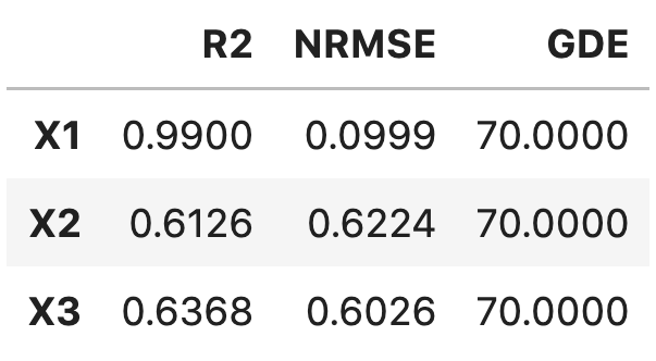
Additionally, the current object of
RegressionAssessmentclass can be compared with another object:from PCAfold import PCA, RegressionAssessment import numpy as np # Generate dummy data set: X = np.random.rand(100,3) Y = np.random.rand(100,3) # Instantiate PCA class object: pca_X = PCA(X, scaling='auto', n_components=2) pca_Y = PCA(Y, scaling='auto', n_components=2) # Approximate the data set: X_rec = pca_X.reconstruct(pca_X.transform(X)) Y_rec = pca_Y.reconstruct(pca_Y.transform(Y)) # Instantiate RegressionAssessment class object: regression_metrics_X = RegressionAssessment(X, X_rec) regression_metrics_Y = RegressionAssessment(Y, Y_rec) # Print regression metrics: regression_metrics_X.print_metrics(table_format=['raw', 'pandas'], float_format='.4f', metrics=['R2', 'NRMSE', 'GDE'], comparison=regression_metrics_Y)
Note
Adding
'raw'to thetable_formatlist will result in printing:------------------------- X1 R2: 0.9133 BETTER NRMSE: 0.2944 BETTER GDE: 67.0000 WORSE ------------------------- X2 R2: 0.5969 WORSE NRMSE: 0.6349 WORSE GDE: 67.0000 WORSE ------------------------- X3 R2: 0.6175 WORSE NRMSE: 0.6185 WORSE GDE: 67.0000 WORSE
Adding
'pandas'to thetable_formatlist (works well in Jupyter notebooks) will result in printing: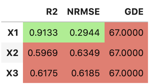
- Parameters:
table_format – (optional)
listofstrspecifying the format(s) in which the table should be printed. Strings can only be'raw','tex'and/or'pandas'.float_format – (optional)
strspecifying the display format for the numerical entries inside the table. By default it is set to'.4f'.metrics – (optional)
listofstrspecifying which metrics should be printed. Strings can only be'R2','MAE','MSE','MSLE','RMSE','NRMSE','GDE'. If metrics is set toNone, all available metrics will be printed.comparison – (optional) object of
RegressionAssessmentclass specifying the metrics that should be compared with the current regression metrics.
- PCAfold.reconstruction.RegressionAssessment.print_stratified_metrics(self, table_format=['raw'], float_format='.4f', metrics=None, comparison=None)
Prints stratified regression assessment metrics as raw text, in
texformat and/or aspandas.DataFrame. In each cluster, in addition to the regression metrics, number of observations is printed, along with the minimum and maximum values of the observed variable in that cluster.Example:
from PCAfold import PCA, variable_bins, RegressionAssessment
import numpy as np

# Generate dummy data set:
X = np.random.rand(100,3)

# Instantiate PCA class object:
pca_X = PCA(X, scaling='auto', n_components=2)

# Approximate the data set:
X_rec = pca_X.reconstruct(pca_X.transform(X))

# Generate bins:
(idx, bins_borders) = variable_bins(X[:,0], k=3, verbose=False)

# Instantiate RegressionAssessment class object:
stratified_regression_metrics = RegressionAssessment(X[:,0], X_rec[:,0], idx=idx)

# Print regression metrics:
stratified_regression_metrics.print_stratified_metrics(table_format=['raw', 'tex', 'pandas'],
                                                       float_format='.4f',
                                                       metrics=['R2', 'MAE', 'NRMSE'])
Note
Adding
'raw'to thetable_formatlist will result in printing:------------------------- k1 Observations: 31 Min: 0.0120 Max: 0.3311 R2: -3.3271 MAE: 0.1774 NRMSE: 2.0802 ------------------------- k2 Observations: 38 Min: 0.3425 Max: 0.6665 R2: -1.4608 MAE: 0.1367 NRMSE: 1.5687 ------------------------- k3 Observations: 31 Min: 0.6853 Max: 0.9959 R2: -3.7319 MAE: 0.1743 NRMSE: 2.1753
Adding
'tex'to thetable_formatlist will result in printing:\begin{table}[h!] \begin{center} \begin{tabular}{llll} \toprule & \textit{k1} & \textit{k2} & \textit{k3} \\ \midrule Observations & 31.0000 & 38.0000 & 31.0000 \\ Min & 0.0120 & 0.3425 & 0.6853 \\ Max & 0.3311 & 0.6665 & 0.9959 \\ R2 & -3.3271 & -1.4608 & -3.7319 \\ MAE & 0.1774 & 0.1367 & 0.1743 \\ NRMSE & 2.0802 & 1.5687 & 2.1753 \\ \end{tabular} \caption{}\label{} \end{center} \end{table}Adding
'pandas'to thetable_formatlist (works well in Jupyter notebooks) will result in printing: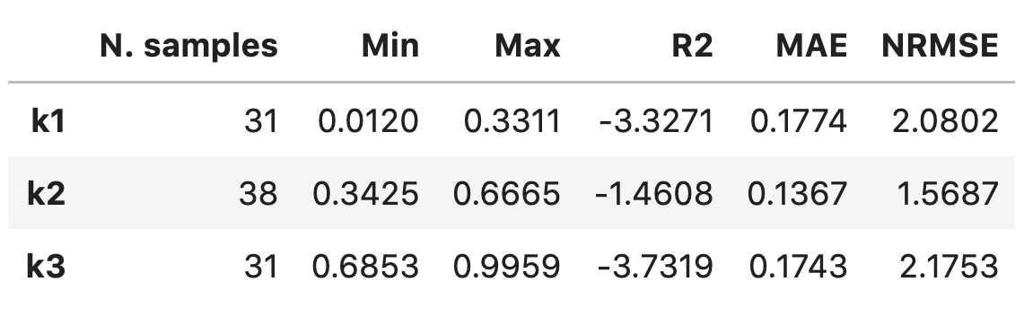
Additionally, the current object of
RegressionAssessmentclass can be compared with another object:from PCAfold import PCA, variable_bins, RegressionAssessment import numpy as np # Generate dummy data set: X = np.random.rand(100,3) # Instantiate PCA class object: pca_X = PCA(X, scaling='auto', n_components=2) # Approximate the data set: X_rec = pca_X.reconstruct(pca_X.transform(X)) # Generate bins: (idx, bins_borders) = variable_bins(X[:,0], k=3, verbose=False) # Instantiate RegressionAssessment class object: stratified_regression_metrics_0 = RegressionAssessment(X[:,0], X_rec[:,0], idx=idx) stratified_regression_metrics_1 = RegressionAssessment(X[:,1], X_rec[:,1], idx=idx) # Print regression metrics: stratified_regression_metrics_0.print_stratified_metrics(table_format=['raw', 'pandas'], float_format='.4f', metrics=['R2', 'MAE', 'NRMSE'], comparison=stratified_regression_metrics_1)
Note
Adding
'raw'to thetable_formatlist will result in printing:------------------------- k1 Observations: 39 Min: 0.0013 Max: 0.3097 R2: 0.9236 BETTER MAE: 0.0185 BETTER NRMSE: 0.2764 BETTER ------------------------- k2 Observations: 29 Min: 0.3519 Max: 0.6630 R2: 0.9380 BETTER MAE: 0.0179 BETTER NRMSE: 0.2491 BETTER ------------------------- k3 Observations: 32 Min: 0.6663 Max: 0.9943 R2: 0.9343 BETTER MAE: 0.0194 BETTER NRMSE: 0.2563 BETTER
Adding
'pandas'to thetable_formatlist (works well in Jupyter notebooks) will result in printing: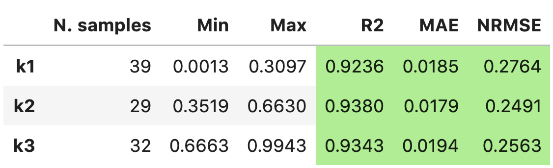
- Parameters:
table_format – (optional)
listofstrspecifying the format(s) in which the table should be printed. Strings can only be'raw','tex'and/or'pandas'.float_format – (optional)
strspecifying the display format for the numerical entries inside the table. By default it is set to'.4f'.metrics – (optional)
listofstrspecifying which metrics should be printed. Strings can only be'R2','MAE','MSE','MSLE','RMSE','NRMSE'. If metrics is set toNone, all available metrics will be printed.comparison – (optional) object of
RegressionAssessmentclass specifying the metrics that should be compared with the current regression metrics.
Regression quality metrics
- PCAfold.reconstruction.coefficient_of_determination(observed, predicted)
Computes the coefficient of determination, \(R^2\), value:
\[R^2 = 1 - \frac{\sum_{i=1}^N (\phi_{o,i} - \phi_{p,i})^2}{\sum_{i=1}^N (\phi_{o,i} - \mathrm{mean}(\phi_{o,i}))^2}\]where \(N\) is the number of observations, \(\phi_o\) is the observed and \(\phi_p\) is the predicted dependent variable.
Example:
from PCAfold import PCA, coefficient_of_determination
import numpy as np

# Generate dummy data set:
X = np.random.rand(100,3)

# Instantiate PCA class object:
pca_X = PCA(X, scaling='auto', n_components=2)

# Approximate the data set:
X_rec = pca_X.reconstruct(pca_X.transform(X))

# Compute the coefficient of determination for the first variable:
r2 = coefficient_of_determination(X[:,0], X_rec[:,0])
- Parameters:
observed –
numpy.ndarrayspecifying the observed values of a single dependent variable, \(\phi_o\). It should be of size(n_observations,)or(n_observations, 1).predicted –
numpy.ndarrayspecifying the predicted values of a single dependent variable, \(\phi_p\). It should be of size(n_observations,)or(n_observations, 1).
- Returns:
r2 - coefficient of determination, \(R^2\).
- PCAfold.reconstruction.stratified_coefficient_of_determination(observed, predicted, idx, use_global_mean=True, verbose=False)
Computes the stratified coefficient of determination, \(R^2\), values. Stratified \(R^2\) is computed separately in each bin (cluster) of an observed dependent variable, \(\phi_o\).
\(R_j^2\) in the \(j^{th}\) bin can be computed in two ways:
If
use_global_mean=True, the mean of the entire observed variable is used as a reference:
\[R_j^2 = 1 - \frac{\sum_{i=1}^{N_j} (\phi_{o,i}^{j} - \phi_{p,i}^{j})^2}{\sum_{i=1}^{N_j} (\phi_{o,i}^{j} - \mathrm{mean}(\phi_o))^2}\]If
use_global_mean=False, the mean of the considered \(j^{th}\) bin is used as a reference:
\[R_j^2 = 1 - \frac{\sum_{i=1}^{N_j} (\phi_{o,i}^{j} - \phi_{p,i}^{j})^2}{\sum_{i=1}^{N_j} (\phi_{o,i}^{j} - \mathrm{mean}(\phi_o^{j}))^2}\]where \(N_j\) is the number of observations in the \(j^{th}\) bin and \(\phi_p\) is the predicted dependent variable.
Note
After running this function you can call
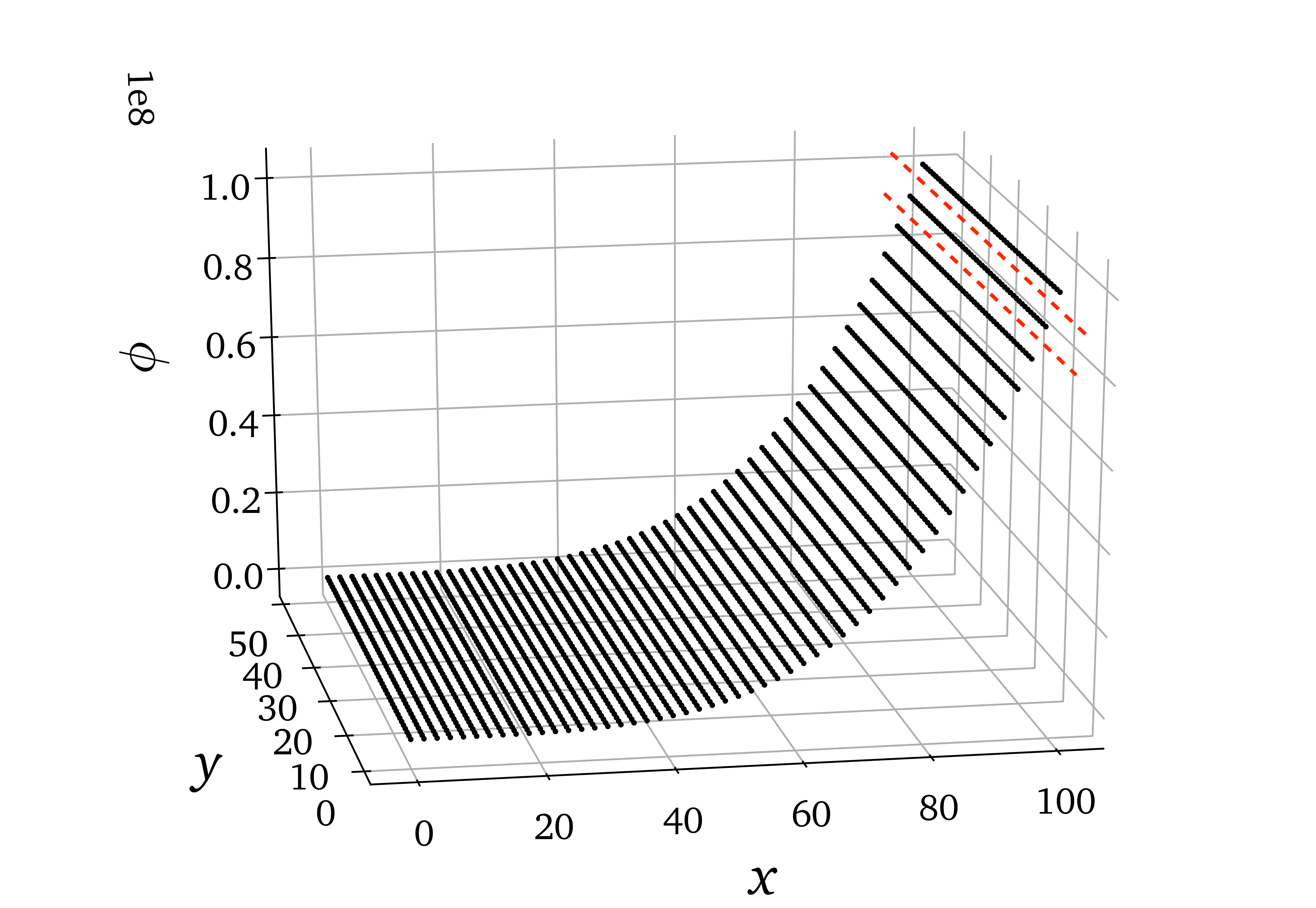
analysis.plot_stratified_coefficient_of_determination(r2_in_bins, bins_borders)on the function outputs and it will visualize how stratified \(R^2\) changes across bins.Warning
The stratified \(R^2\) metric can be misleading if there are large variations in point density in an observed variable. For instance, below is a data set composed of lines of points that have uniform spacing on the \(x\) axis but become more and more sparse in the direction of increasing \(\phi\) due to an increasing gradient of \(\phi\). If bins are narrow enough (number of bins is high enough), a single bin (like the bin bounded by the red dashed lines) can contain only one of those lines of points for high value of \(\phi\). \(R^2\) will then be computed for constant, or almost constant observations, even though globally those observations lie in a location of a large gradient of the observed variable!
Example:
from PCAfold import PCA, variable_bins, stratified_coefficient_of_determination, plot_stratified_coefficient_of_determination
import numpy as np

# Generate dummy data set:
X = np.random.rand(100,10)

# Instantiate PCA class object:
pca_X = PCA(X, scaling='auto', n_components=2)

# Approximate the data set:
X_rec = pca_X.reconstruct(pca_X.transform(X))

# Generate bins:
(idx, bins_borders) = variable_bins(X[:,0], k=10, verbose=False)

# Compute stratified R2 in 10 bins of the first variable in a data set:
r2_in_bins = stratified_coefficient_of_determination(X[:,0],
                                                     X_rec[:,0],
                                                     idx=idx,
                                                     use_global_mean=True,
                                                     verbose=True)

# Plot the stratified R2 values:
plot_stratified_coefficient_of_determination(r2_in_bins, bins_borders)
- Parameters:
observed –
numpy.ndarrayspecifying the observed values of a single dependent variable, \(\phi_o\). It should be of size(n_observations,)or(n_observations, 1).predicted –
numpy.ndarrayspecifying the predicted values of a single dependent variable, \(\phi_p\). It should be of size(n_observations,)or(n_observations, 1).idx –
numpy.ndarrayof cluster classifications. It should be of size(n_observations,)or(n_observations,1).use_global_mean – (optional)
boolspecifying if global mean of the observed variable should be used as a reference in \(R^2\) calculation.verbose – (optional)
boolfor printing sizes (number of observations) and \(R^2\) values in each bin.
- Returns:
r2_in_bins -
listspecifying the coefficients of determination \(R^2\) in each bin. It has lengthk.
- PCAfold.reconstruction.mean_absolute_error(observed, predicted)
Computes the mean absolute error (MAE):
\[\mathrm{MAE} = \frac{1}{N} \sum_{i=1}^N | \phi_{o,i} - \phi_{p,i} |\]where \(N\) is the number of observations, \(\phi_o\) is the observed and \(\phi_p\) is the predicted dependent variable.
Example:
from PCAfold import PCA, mean_absolute_error
import numpy as np

# Generate dummy data set:
X = np.random.rand(100,3)

# Instantiate PCA class object:
pca_X = PCA(X, scaling='auto', n_components=2)

# Approximate the data set:
X_rec = pca_X.reconstruct(pca_X.transform(X))

# Compute the mean absolute error for the first variable:
mae = mean_absolute_error(X[:,0], X_rec[:,0])
- Parameters:
observed –
numpy.ndarrayspecifying the observed values of a single dependent variable, \(\phi_o\). It should be of size(n_observations,)or(n_observations, 1).predicted –
numpy.ndarrayspecifying the predicted values of a single dependent variable, \(\phi_p\). It should be of size(n_observations,)or(n_observations, 1).
- Returns:
mae - mean absolute error (MAE).
- PCAfold.reconstruction.stratified_mean_absolute_error(observed, predicted, idx, verbose=False)
Computes the stratified mean absolute error (MAE) values. Stratified MAE is computed separately in each bin (cluster) of an observed dependent variable, \(\phi_o\).
MAE in the \(j^{th}\) bin can be computed as:
\[\mathrm{MAE}_j = \frac{1}{N_j} \sum_{i=1}^{N_j} | \phi_{o,i}^j - \phi_{p,i}^j |\]where \(N_j\) is the number of observations in the \(j^{th}\) bin, \(\phi_o\) is the observed and \(\phi_p\) is the predicted dependent variable.
Example:
from PCAfold import PCA, variable_bins, stratified_mean_absolute_error
import numpy as np

# Generate dummy data set:
X = np.random.rand(100,10)

# Instantiate PCA class object:
pca_X = PCA(X, scaling='auto', n_components=2)

# Approximate the data set:
X_rec = pca_X.reconstruct(pca_X.transform(X))

# Generate bins:
(idx, bins_borders) = variable_bins(X[:,0], k=10, verbose=False)

# Compute stratified MAE in 10 bins of the first variable in a data set:
mae_in_bins = stratified_mean_absolute_error(X[:,0],
                                             X_rec[:,0],
                                             idx=idx,
                                             verbose=True)
- Parameters:
observed –
numpy.ndarrayspecifying the observed values of a single dependent variable, \(\phi_o\). It should be of size(n_observations,)or(n_observations, 1).predicted –
numpy.ndarrayspecifying the predicted values of a single dependent variable, \(\phi_p\). It should be of size(n_observations,)or(n_observations, 1).idx –
numpy.ndarrayof cluster classifications. It should be of size(n_observations,)or(n_observations,1).verbose – (optional)
boolfor printing sizes (number of observations) and MAE values in each bin.
- Returns:
mae_in_bins -
listspecifying the mean absolute error (MAE) in each bin. It has lengthk.
- PCAfold.reconstruction.max_absolute_error(observed, predicted)
Computes the maximum absolute error (MaxAE):
\[\mathrm{MaxAE} = \mathrm{max}( | \phi_{o,i} - \phi_{p,i} | )\]where \(\phi_o\) is the observed and \(\phi_p\) is the predicted dependent variable.
Example:
from PCAfold import PCA, max_absolute_error
import numpy as np

# Generate dummy data set:
X = np.random.rand(100,3)

# Instantiate PCA class object:
pca_X = PCA(X, scaling='auto', n_components=2)

# Approximate the data set:
X_rec = pca_X.reconstruct(pca_X.transform(X))

# Compute the maximum absolute error for the first variable:
maxae = max_absolute_error(X[:,0], X_rec[:,0])
- Parameters:
observed –
numpy.ndarrayspecifying the observed values of a single dependent variable, \(\phi_o\). It should be of size(n_observations,)or(n_observations, 1).predicted –
numpy.ndarrayspecifying the predicted values of a single dependent variable, \(\phi_p\). It should be of size(n_observations,)or(n_observations, 1).
- Returns:
maxae - max absolute error (MaxAE).
- PCAfold.reconstruction.stratified_max_absolute_error(observed, predicted, idx, verbose=False)
Computes the stratified max absolute error (MaxAE) values. Stratified MaxAE is computed separately in each bin (cluster) of an observed dependent variable, \(\phi_o\).
MaxAE in the \(j^{th}\) bin can be computed as:
\[\mathrm{MaxAE}_j = \mathrm{max}( | \phi_{o,i}^j - \phi_{p,i}^j | )\]where \(\phi_o\) is the observed and \(\phi_p\) is the predicted dependent variable.
Example:
from PCAfold import PCA, variable_bins, stratified_max_absolute_error
import numpy as np

# Generate dummy data set:
X = np.random.rand(100,10)

# Instantiate PCA class object:
pca_X = PCA(X, scaling='auto', n_components=2)

# Approximate the data set:
X_rec = pca_X.reconstruct(pca_X.transform(X))

# Generate bins:
(idx, bins_borders) = variable_bins(X[:,0], k=10, verbose=False)

# Compute stratified MaxAE in 10 bins of the first variable in a data set:
maxae_in_bins = stratified_max_absolute_error(X[:,0],
                                              X_rec[:,0],
                                              idx=idx,
                                              verbose=True)
- Parameters:
observed –
numpy.ndarrayspecifying the observed values of a single dependent variable, \(\phi_o\). It should be of size(n_observations,)or(n_observations, 1).predicted –
numpy.ndarrayspecifying the predicted values of a single dependent variable, \(\phi_p\). It should be of size(n_observations,)or(n_observations, 1).idx –
numpy.ndarrayof cluster classifications. It should be of size(n_observations,)or(n_observations,1).verbose – (optional)
boolfor printing sizes (number of observations) and MSE values in each bin.
- Returns:
maxae_in_bins -
listspecifying the max absolute error (MaxAE) in each bin. It has lengthk.
- PCAfold.reconstruction.mean_squared_error(observed, predicted)
Computes the mean squared error (MSE):
\[\mathrm{MSE} = \frac{1}{N} \sum_{i=1}^N (\phi_{o,i} - \phi_{p,i}) ^2\]where \(N\) is the number of observations, \(\phi_o\) is the observed and \(\phi_p\) is the predicted dependent variable.
Example:
from PCAfold import PCA, mean_squared_error
import numpy as np

# Generate dummy data set:
X = np.random.rand(100,3)

# Instantiate PCA class object:
pca_X = PCA(X, scaling='auto', n_components=2)

# Approximate the data set:
X_rec = pca_X.reconstruct(pca_X.transform(X))

# Compute the mean squared error for the first variable:
mse = mean_squared_error(X[:,0], X_rec[:,0])
- Parameters:
observed –
numpy.ndarrayspecifying the observed values of a single dependent variable, \(\phi_o\). It should be of size(n_observations,)or(n_observations, 1).predicted –
numpy.ndarrayspecifying the predicted values of a single dependent variable, \(\phi_p\). It should be of size(n_observations,)or(n_observations, 1).
- Returns:
mse - mean squared error (MSE).
- PCAfold.reconstruction.stratified_mean_squared_error(observed, predicted, idx, verbose=False)
Computes the stratified mean squared error (MSE) values. Stratified MSE is computed separately in each bin (cluster) of an observed dependent variable, \(\phi_o\).
MSE in the \(j^{th}\) bin can be computed as:
\[\mathrm{MSE}_j = \frac{1}{N_j} \sum_{i=1}^{N_j} (\phi_{o,i}^j - \phi_{p,i}^j) ^2\]where \(N_j\) is the number of observations in the \(j^{th}\) bin, \(\phi_o\) is the observed and \(\phi_p\) is the predicted dependent variable.
Example:
from PCAfold import PCA, variable_bins, stratified_mean_squared_error
import numpy as np

# Generate dummy data set:
X = np.random.rand(100,10)

# Instantiate PCA class object:
pca_X = PCA(X, scaling='auto', n_components=2)

# Approximate the data set:
X_rec = pca_X.reconstruct(pca_X.transform(X))

# Generate bins:
(idx, bins_borders) = variable_bins(X[:,0], k=10, verbose=False)

# Compute stratified MSE in 10 bins of the first variable in a data set:
mse_in_bins = stratified_mean_squared_error(X[:,0],
                                            X_rec[:,0],
                                            idx=idx,
                                            verbose=True)
- Parameters:
observed –
numpy.ndarrayspecifying the observed values of a single dependent variable, \(\phi_o\). It should be of size(n_observations,)or(n_observations, 1).predicted –
numpy.ndarrayspecifying the predicted values of a single dependent variable, \(\phi_p\). It should be of size(n_observations,)or(n_observations, 1).idx –
numpy.ndarrayof cluster classifications. It should be of size(n_observations,)or(n_observations,1).verbose – (optional)
boolfor printing sizes (number of observations) and MSE values in each bin.
- Returns:
mse_in_bins -
listspecifying the mean squared error (MSE) in each bin. It has lengthk.
- PCAfold.reconstruction.mean_squared_logarithmic_error(observed, predicted)
Computes the mean squared logarithmic error (MSLE):
\[\mathrm{MSLE} = \frac{1}{N} \sum_{i=1}^N (\log(\phi_{o,i} + 1) - \log(\phi_{p,i} + 1)) ^2\]where \(N\) is the number of observations, \(\phi_o\) is the observed and \(\phi_p\) is the predicted dependent variable.
Warning
The MSLE metric can only be used on non-negative samples.
Example:
from PCAfold import PCA, mean_squared_logarithmic_error
import numpy as np

# Generate dummy data set:
X = np.random.rand(100,3)

# Instantiate PCA class object:
pca_X = PCA(X, scaling='auto', n_components=2)

# Approximate the data set:
X_rec = pca_X.reconstruct(pca_X.transform(X))

# Compute the mean squared error for the first variable:
msle = mean_squared_logarithmic_error(X[:,0], X_rec[:,0])
- Parameters:
observed –
numpy.ndarrayspecifying the observed values of a single dependent variable, \(\phi_o\). It should be of size(n_observations,)or(n_observations, 1).predicted –
numpy.ndarrayspecifying the predicted values of a single dependent variable, \(\phi_p\). It should be of size(n_observations,)or(n_observations, 1).
- Returns:
msle - mean squared logarithmic error (MSLE).
- PCAfold.reconstruction.stratified_mean_squared_logarithmic_error(observed, predicted, idx, verbose=False)
Computes the stratified mean squared logarithmic error (MSLE) values. Stratified MSLE is computed separately in each bin (cluster) of an observed dependent variable, \(\phi_o\).
MSLE in the \(j^{th}\) bin can be computed as:
\[\mathrm{MSLE}_j = \frac{1}{N_j} \sum_{i=1}^{N_j} (\log(\phi_{o,i}^j + 1) - \log(\phi_{p,i}^j + 1)) ^2\]where \(N_j\) is the number of observations in the \(j^{th}\) bin, \(\phi_o\) is the observed and \(\phi_p\) is the predicted dependent variable.
Warning
The MSLE metric can only be used on non-negative samples.
Example:
from PCAfold import PCA, variable_bins, stratified_mean_squared_logarithmic_error
import numpy as np

# Generate dummy data set:
X = np.random.rand(100,10)

# Instantiate PCA class object:
pca_X = PCA(X, scaling='auto', n_components=2)

# Approximate the data set:
X_rec = pca_X.reconstruct(pca_X.transform(X))

# Generate bins:
(idx, bins_borders) = variable_bins(X[:,0], k=10, verbose=False)

# Compute stratified MSLE in 10 bins of the first variable in a data set:
msle_in_bins = stratified_mean_squared_logarithmic_error(X[:,0],
                                                         X_rec[:,0],
                                                         idx=idx,
                                                         verbose=True)
- Parameters:
observed –
numpy.ndarrayspecifying the observed values of a single dependent variable, \(\phi_o\). It should be of size(n_observations,)or(n_observations, 1).predicted –
numpy.ndarrayspecifying the predicted values of a single dependent variable, \(\phi_p\). It should be of size(n_observations,)or(n_observations, 1).idx –
numpy.ndarrayof cluster classifications. It should be of size(n_observations,)or(n_observations,1).verbose – (optional)
boolfor printing sizes (number of observations) and MSLE values in each bin.
- Returns:
msle_in_bins -
listspecifying the mean squared logarithmic error (MSLE) in each bin. It has lengthk.
- PCAfold.reconstruction.root_mean_squared_error(observed, predicted)
Computes the root mean squared error (RMSE):
\[\mathrm{RMSE} = \sqrt{\frac{1}{N} \sum_{i=1}^N (\phi_{o,i} - \phi_{p,i}) ^2}\]where \(N\) is the number of observations, \(\phi_o\) is the observed and \(\phi_p\) is the predicted dependent variable.
Example:
from PCAfold import PCA, root_mean_squared_error
import numpy as np

# Generate dummy data set:
X = np.random.rand(100,3)

# Instantiate PCA class object:
pca_X = PCA(X, scaling='auto', n_components=2)

# Approximate the data set:
X_rec = pca_X.reconstruct(pca_X.transform(X))

# Compute the root mean squared error for the first variable:
rmse = root_mean_squared_error(X[:,0], X_rec[:,0])
- Parameters:
observed –
numpy.ndarrayspecifying the observed values of a single dependent variable, \(\phi_o\). It should be of size(n_observations,)or(n_observations, 1).predicted –
numpy.ndarrayspecifying the predicted values of a single dependent variable, \(\phi_p\). It should be of size(n_observations,)or(n_observations, 1).
- Returns:
rmse - root mean squared error (RMSE).
- PCAfold.reconstruction.stratified_root_mean_squared_error(observed, predicted, idx, verbose=False)
Computes the stratified root mean squared error (RMSE) values. Stratified RMSE is computed separately in each bin (cluster) of an observed dependent variable, \(\phi_o\).
RMSE in the \(j^{th}\) bin can be computed as:
\[\mathrm{RMSE}_j = \sqrt{\frac{1}{N_j} \sum_{i=1}^{N_j} (\phi_{o,i}^j - \phi_{p,i}^j) ^2}\]where \(N_j\) is the number of observations in the \(j^{th}\) bin, \(\phi_o\) is the observed and \(\phi_p\) is the predicted dependent variable.
Example:
from PCAfold import PCA, variable_bins, stratified_root_mean_squared_error
import numpy as np

# Generate dummy data set:
X = np.random.rand(100,10)

# Instantiate PCA class object:
pca_X = PCA(X, scaling='auto', n_components=2)

# Approximate the data set:
X_rec = pca_X.reconstruct(pca_X.transform(X))

# Generate bins:
(idx, bins_borders) = variable_bins(X[:,0], k=10, verbose=False)

# Compute stratified RMSE in 10 bins of the first variable in a data set:
rmse_in_bins = stratified_root_mean_squared_error(X[:,0],
                                                  X_rec[:,0],
                                                  idx=idx,
                                                  verbose=True)
- Parameters:
observed –
numpy.ndarrayspecifying the observed values of a single dependent variable, \(\phi_o\). It should be of size(n_observations,)or(n_observations, 1).predicted –
numpy.ndarrayspecifying the predicted values of a single dependent variable, \(\phi_p\). It should be of size(n_observations,)or(n_observations, 1).idx –
numpy.ndarrayof cluster classifications. It should be of size(n_observations,)or(n_observations,1).verbose – (optional)
boolfor printing sizes (number of observations) and RMSE values in each bin.
- Returns:
rmse_in_bins -
listspecifying the mean squared error (RMSE) in each bin. It has lengthk.
- PCAfold.reconstruction.normalized_root_mean_squared_error(observed, predicted, norm='std')
Computes the normalized root mean squared error (NRMSE):
\[\mathrm{NRMSE} = \frac{1}{d_{norm}} \sqrt{\frac{1}{N} \sum_{i=1}^N (\phi_{o,i} - \phi_{p,i}) ^2}\]where \(d_{norm}\) is the normalization factor, \(N\) is the number of observations, \(\phi_o\) is the observed and \(\phi_p\) is the predicted dependent variable.
Various normalizations are available:
Normalization
normNormalization factor \(d_{norm}\)
Root square mean
'root_square_mean'\(d_{norm} = \sqrt{\mathrm{mean}(\phi_o^2)}\)
Std
'std'\(d_{norm} = \mathrm{std}(\phi_o)\)
Range
'range'\(d_{norm} = \mathrm{max}(\phi_o) - \mathrm{min}(\phi_o)\)
Root square range
'root_square_range'\(d_{norm} = \sqrt{\mathrm{max}(\phi_o^2) - \mathrm{min}(\phi_o^2)}`\)
Root square std
'root_square_std'\(d_{norm} = \sqrt{\mathrm{std}(\phi_o^2)}\)
Absolute mean
'abs_mean'\(d_{norm} = | \mathrm{mean}(\phi_o) |\)
Example:
from PCAfold import PCA, normalized_root_mean_squared_error
import numpy as np

# Generate dummy data set:
X = np.random.rand(100,3)

# Instantiate PCA class object:
pca_X = PCA(X, scaling='auto', n_components=2)

# Approximate the data set:
X_rec = pca_X.reconstruct(pca_X.transform(X))

# Compute the root mean squared error for the first variable:
nrmse = normalized_root_mean_squared_error(X[:,0], X_rec[:,0], norm='std')
- Parameters:
observed –
numpy.ndarrayspecifying the observed values of a single dependent variable, \(\phi_o\). It should be of size(n_observations,)or(n_observations, 1).predicted –
numpy.ndarrayspecifying the predicted values of a single dependent variable, \(\phi_p\). It should be of size(n_observations,)or(n_observations, 1).norm –
strspecifying the normalization, \(d_{norm}\). It can be one of the following:std,range,root_square_mean,root_square_range,root_square_std,abs_mean.
- Returns:
nrmse - normalized root mean squared error (NRMSE).
- PCAfold.reconstruction.stratified_normalized_root_mean_squared_error(observed, predicted, idx, norm='std', use_global_norm=False, verbose=False)
Computes the stratified normalized root mean squared error (NRMSE) values. Stratified NRMSE is computed separately in each bin (cluster) of an observed dependent variable, \(\phi_o\).
NRMSE in the \(j^{th}\) bin can be computed as:
\[\mathrm{NRMSE}_j = \frac{1}{d_{norm}} \sqrt{\frac{1}{N_j} \sum_{i=1}^{N_j} (\phi_{o,i}^j - \phi_{p,i}^j) ^2}\]where \(N_j\) is the number of observations in the \(j^{th}\) bin, \(\phi_o\) is the observed and \(\phi_p\) is the predicted dependent variable.
Example:
from PCAfold import PCA, variable_bins, stratified_normalized_root_mean_squared_error
import numpy as np

# Generate dummy data set:
X = np.random.rand(100,10)

# Instantiate PCA class object:
pca_X = PCA(X, scaling='auto', n_components=2)

# Approximate the data set:
X_rec = pca_X.reconstruct(pca_X.transform(X))

# Generate bins:
(idx, bins_borders) = variable_bins(X[:,0], k=10, verbose=False)

# Compute stratified NRMSE in 10 bins of the first variable in a data set:
nrmse_in_bins = stratified_normalized_root_mean_squared_error(X[:,0],
                                                              X_rec[:,0],
                                                              idx=idx,
                                                              norm='std',
                                                              use_global_norm=True,
                                                              verbose=True)
- Parameters:
observed –
numpy.ndarrayspecifying the observed values of a single dependent variable, \(\phi_o\). It should be of size(n_observations,)or(n_observations, 1).predicted –
numpy.ndarrayspecifying the predicted values of a single dependent variable, \(\phi_p\). It should be of size(n_observations,)or(n_observations, 1).idx –
numpy.ndarrayof cluster classifications. It should be of size(n_observations,)or(n_observations,1).norm –
strspecifying the normalization, \(d_{norm}\). It can be one of the following:std,range,root_square_mean,root_square_range,root_square_std,abs_mean.use_global_norm – (optional)
boolspecifying if global norm of the observed variable should be used in NRMSE calculation. If set toFalse, norms are computed on samples from the the corresponding bin.verbose – (optional)
boolfor printing sizes (number of observations) and NRMSE values in each bin.
- Returns:
nrmse_in_bins -
listspecifying the mean squared error (NRMSE) in each bin. It has lengthk.
- PCAfold.reconstruction.turning_points(observed, predicted)
Computes the turning points percentage - the percentage of predicted outputs that have the opposite growth tendency to the corresponding observed growth tendency.
Warning
This function is under construction.
- Returns:
turning_points - turning points percentage in %.
- PCAfold.reconstruction.good_estimate(observed, predicted, tolerance=0.05)
Computes the good estimate (GE) - the percentage of predicted values that are within the specified tolerance from the corresponding observed values.
Warning
This function is under construction.
- Parameters:
observed –
numpy.ndarrayspecifying the observed values of a single dependent variable. It should be of size(n_observations,)or(n_observations, 1).predicted –
numpy.ndarrayspecifying the predicted values of a single dependent variable. It should be of size(n_observations,)or(n_observations, 1).
- Parm tolerance:
floatspecifying the tolerance.- Returns:
good_estimate - good estimate (GE) in %.
- PCAfold.reconstruction.good_direction_estimate(observed, predicted, tolerance=0.05)
Computes the good direction (GD) and the good direction estimate (GDE).
GD for observation \(i\), is computed as:
\[GD_i = \frac{\vec{\phi}_{o,i}}{|| \vec{\phi}_{o,i} ||} \cdot \frac{\vec{\phi}_{p,i}}{|| \vec{\phi}_{p,i} ||}\]where \(\vec{\phi}_o\) is the observed vector quantity and \(\vec{\phi}_p\) is the predicted vector quantity.
GDE is computed as the percentage of predicted vector observations whose direction is within the specified tolerance from the direction of the corresponding observed vector.
Example:
from PCAfold import PCA, good_direction_estimate
import numpy as np

# Generate dummy data set:
X = np.random.rand(100,3)

# Instantiate PCA class object:
pca_X = PCA(X, scaling='auto', n_components=2)

# Approximate the data set:
X_rec = pca_X.reconstruct(pca_X.transform(X))

# Compute the vector of good direction and good direction estimate:
(good_direction, good_direction_estimate) = good_direction_estimate(X,
                                                                    X_rec,
                                                                    tolerance=0.01)
- Parameters:
observed –
numpy.ndarrayspecifying the observed vector quantity, \(\vec{\phi}_o\). It should be of size(n_observations,n_dimensions).predicted –
numpy.ndarrayspecifying the predicted vector quantity, \(\vec{\phi}_p\). It should be of size(n_observations,n_dimensions).tolerance –
floatspecifying the tolerance.
- Returns:
good_direction -
numpy.ndarrayspecifying the vector of good direction (GD). It has size(n_observations,).good_direction_estimate - good direction estimate (GDE) in %.
- PCAfold.reconstruction.generate_tex_table(data_frame_table, float_format='.2f', caption='', label='')
Generates
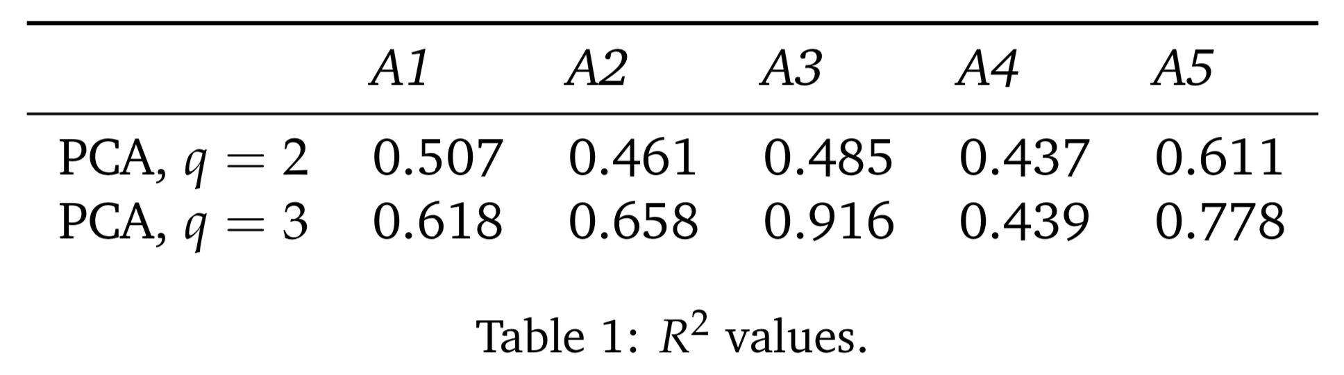
texcode for a table stored in apandas.DataFrame. This function can be useful e.g. for printing regression results.Example:
from PCAfold import PCA, generate_tex_table
import numpy as np
import pandas as pd

# Generate dummy data set:
X = np.random.rand(100,5)

# Generate dummy variables names:
variable_names = ['A1', 'A2', 'A3', 'A4', 'A5']

# Instantiate PCA class object:
pca_q2 = PCA(X, scaling='auto', n_components=2, use_eigendec=True, nocenter=False)
pca_q3 = PCA(X, scaling='auto', n_components=3, use_eigendec=True, nocenter=False)

# Calculate the R2 values:
r2_q2 = pca_q2.calculate_r2(X)[None,:]
r2_q3 = pca_q3.calculate_r2(X)[None,:]

# Generate pandas.DataFrame from the R2 values:
r2_table = pd.DataFrame(np.vstack((r2_q2, r2_q3)),
                        columns=variable_names,
                        index=['PCA, $q=2$', 'PCA, $q=3$'])

# Generate tex code for the table:
generate_tex_table(r2_table,
                   float_format=".3f",
                   caption='$R^2$ values.',
                   label='r2-values')
Note
The code above will produce
texcode:\begin{table}[h!] \begin{center} \begin{tabular}{llllll} \toprule & \textit{A1} & \textit{A2} & \textit{A3} & \textit{A4} & \textit{A5} \\ \midrule PCA, $q=2$ & 0.507 & 0.461 & 0.485 & 0.437 & 0.611 \\ PCA, $q=3$ & 0.618 & 0.658 & 0.916 & 0.439 & 0.778 \\ \end{tabular} \caption{$R^2$ values.}\label{r2-values} \end{center} \end{table}Which, when compiled, will result in a table:
- Parameters:
data_frame_table –
pandas.DataFramespecifying the table to convert totexcode. It can include column names and index names.float_format –
strspecifying the display format for the numerical entries inside the table. By default it is set to'.2f'.caption –
strspecifying caption for the table.label –
strspecifying label for the table.
Plotting functions
- PCAfold.reconstruction.plot_2d_regression(x, observed, predicted, x_label=None, y_label=None, color_observed=None, color_predicted=None, figure_size=(7, 7), title=None, save_filename=None)
Plots the result of regression of a dependent variable on top of a one-dimensional manifold defined by a single independent variable
x.Example:
from PCAfold import PCA, plot_2d_regression
import numpy as np

# Generate dummy data set:
X = np.random.rand(100,10)

# Obtain two-dimensional manifold from PCA:
pca_X = PCA(X)
PCs = pca_X.transform(X)
X_rec = pca_X.reconstruct(PCs)

# Plot the manifold:
plt = plot_2d_regression(X[:,0],
                         X[:,0],
                         X_rec[:,0],
                         x_label='$x$',
                         y_label='$y$',
                         color_observed='k',
                         color_predicted='r',
                         figure_size=(10,10),
                         title='2D regression',
                         save_filename='2d-regression.pdf')
plt.close()
- Parameters:
x –
numpy.ndarrayspecifying the variable on the \(x\)-axis. It should be of size(n_observations,)or(n_observations,1).observed –
numpy.ndarrayspecifying the observed values of a single dependent variable. It should be of size(n_observations,)or(n_observations, 1).predicted –
numpy.ndarrayspecifying the predicted values of a single dependent variable. It should be of size(n_observations,)or(n_observations, 1).x_label – (optional)
strspecifying \(x\)-axis label annotation. If set toNonelabel will not be plotted.y_label – (optional)
strspecifying \(y\)-axis label annotation. If set toNonelabel will not be plotted.color_observed – (optional)
strspecifying the color of the plotted observed variable.color_predicted – (optional)
strspecifying the color of the plotted predicted variable.figure_size – (optional)
tuplespecifying figure size.title – (optional)
strspecifying plot title. If set toNonetitle will not be plotted.save_filename – (optional)
strspecifying plot save location/filename. If set toNoneplot will not be saved. You can also set a desired file extension, for instance.pdf. If the file extension is not specified, the default is.png.
- Returns:
plt -
matplotlib.pyplotplot handle.
- PCAfold.reconstruction.plot_2d_regression_scalar_field(grid_bounds, regression_model, x=None, y=None, resolution=(10, 10), extension=(0, 0), x_label=None, y_label=None, s_field=None, s_manifold=None, manifold_color=None, colorbar_label=None, color_map='viridis', colorbar_range=None, manifold_alpha=1, grid_on=True, figure_size=(7, 7), title=None, save_filename=None)
Plots a 2D field of a regressed scalar dependent variable. A two-dimensional manifold can be additionally plotted on top of the field.
Example:
from PCAfold import PCA, KReg, plot_2d_regression_scalar_field
import numpy as np

# Generate dummy data set:
X = np.random.rand(100,2)
Z = np.random.rand(100,1)

# Train the kernel regression model:
model = KReg(X, Z)

# Define the regression model:
def regression_model(query):

    predicted = model.predict(query, 'nearest_neighbors_isotropic', n_neighbors=1)[0,0]

    return predicted

# Define the bounds for the scalar field:
grid_bounds = ([np.min(X[:,0]),np.max(X[:,0])],[np.min(X[:,1]),np.max(X[:,1])])

# Plot the regressed scalar field:
plt = plot_2d_regression_scalar_field(grid_bounds,
                                      regression_model,
                                      x=X[:,0],
                                      y=X[:,1],
                                      resolution=(100,100),
                                      extension=(10,10),
                                      x_label='$X_1$',
                                      y_label='$X_2$',
                                      s_field=4,
                                      s_manifold=60,
                                      manifold_color=Z,
                                      colorbar_label='$Z_1$',
                                      color_map='inferno',
                                      colorbar_range=(0,1),
                                      manifold_alpha=1,
                                      grid_on=False,
                                      figure_size=(10,6),
                                      title='2D regressed scalar field',
                                      save_filename='2D-regressed-scalar-field.pdf')
plt.close()
- Parameters:
grid_bounds –
tupleoflistspecifying the bounds of the dependent variable on the \(x\) and \(y\) axis.regression_model –
functionthat outputs the predicted vector using the regression model. It should take as input anumpy.ndarrayof size(1,2), where the two elements specify the first and second independent variable values. It should output afloatspecifying the regressed scalar value at that input.x – (optional)
numpy.ndarrayspecifying the variable on the \(x\)-axis. It should be of size(n_observations,)or(n_observations,1). It can be used to plot a 2D manifold on top of the streamplot.y – (optional)
numpy.ndarrayspecifying the variable on the \(y\)-axis. It should be of size(n_observations,)or(n_observations,1). It can be used to plot a 2D manifold on top of the streamplot.resolution – (optional)
tupleofintspecifying the resolution of the streamplot grid on the \(x\) and \(y\) axis.extension – (optional)
tupleoffloatorintspecifying a percentage by which the dependent variable should be extended beyond on the \(x\) and \(y\) axis, beyond what has been specified by thegrid_boundsparameter.x_label – (optional)
strspecifying \(x\)-axis label annotation. If set toNonelabel will not be plotted.y_label – (optional)
strspecifying \(y\)-axis label annotation. If set toNonelabel will not be plotted.s_field – (optional)
intorfloatspecifying the scatter point size for the scalar field.s_manifold – (optional)
intorfloatspecifying the scatter point size for the manifold.manifold_color – (optional) vector or string specifying color for the manifold. If it is a vector, it has to have length consistent with the number of observations in
xandyvectors. It should be of typenumpy.ndarrayand size(n_observations,)or(n_observations,1). It can also be set to a string specifying the color directly, for instance'r'or'#006778'. If not specified, manifold will be plotted in black.colorbar_label – (optional)
strspecifying colorbar label annotation.color_map – (optional)
strormatplotlib.colors.ListedColormapspecifying the colormap to use as permatplotlib.cm. Default is'viridis'.colorbar_range – (optional)
tuplespecifying the lower and the upper bound for the colorbar range.manifold_alpha – (optional)
floatorintspecifying the opacity of the plotted manifold.grid_on –
boolspecifying whether grid should be plotted.figure_size – (optional)
tuplespecifying figure size.title – (optional)
strspecifying plot title. If set toNonetitle will not be plotted.save_filename – (optional)
strspecifying plot save location/filename. If set toNoneplot will not be saved. You can also set a desired file extension, for instance.pdf. If the file extension is not specified, the default is.png.
- Returns:
plt -
matplotlib.pyplotplot handle.
- PCAfold.reconstruction.plot_2d_regression_streamplot(grid_bounds, regression_model, x=None, y=None, resolution=(10, 10), extension=(0, 0), color='k', x_label=None, y_label=None, s_manifold=None, manifold_color=None, colorbar_label=None, color_map='viridis', colorbar_range=None, manifold_alpha=1, grid_on=True, figure_size=(7, 7), title=None, save_filename=None)
Plots a streamplot of a regressed vector field of a dependent variable. A two-dimensional manifold can be additionally plotted on top of the streamplot.
Example:
from PCAfold import PCA, KReg, plot_2d_regression_streamplot
import numpy as np

# Generate dummy data set:
X = np.random.rand(100,5)
S_X = np.random.rand(100,5)

# Obtain two-dimensional manifold from PCA:
pca_X = PCA(X, n_components=2)
PCs = pca_X.transform(X)
S_Z = pca_X.transform(S_X, nocenter=True)

# Train the kernel regression model:
model = KReg(PCs, S_Z)

# Define the regression model:
def regression_model(query):

    predicted = model.predict(query, 'nearest_neighbors_isotropic', n_neighbors=1)

    return predicted

# Define the bounds for the streamplot:
grid_bounds = ([np.min(PCs[:,0]),np.max(PCs[:,0])],[np.min(PCs[:,1]),np.max(PCs[:,1])])

# Plot the regression streamplot:
plt = plot_2d_regression_streamplot(grid_bounds,
                                    regression_model,
                                    x=PCs[:,0],
                                    y=PCs[:,1],
                                    resolution=(15,15),
                                    extension=(20,20),
                                    color='r',
                                    x_label='$Z_1$',
                                    y_label='$Z_2$',
                                    manifold_color=X[:,0],
                                    colorbar_label='$X_1$',
                                    color_map='plasma',
                                    colorbar_range=(0,1),
                                    manifold_alpha=1,
                                    grid_on=False,
                                    figure_size=(10,6),
                                    title='Streamplot',
                                    save_filename='streamplot.pdf')
plt.close()
- Parameters:
grid_bounds –
tupleoflistspecifying the bounds of the dependent variable on the \(x\) and \(y\) axis.regression_model –
functionthat outputs the predicted vector using the regression model. It should take as input anumpy.ndarrayof size(1,2), where the two elements specify the first and second independent variable values. It should output anumpy.ndarrayof size(1,2), where the two elements specify the first and second regressed vector elements.x – (optional)
numpy.ndarrayspecifying the variable on the \(x\)-axis. It should be of size(n_observations,)or(n_observations,1). It can be used to plot a 2D manifold on top of the streamplot.y – (optional)
numpy.ndarrayspecifying the variable on the \(y\)-axis. It should be of size(n_observations,)or(n_observations,1). It can be used to plot a 2D manifold on top of the streamplot.resolution – (optional)
tupleofintspecifying the resolution of the streamplot grid on the \(x\) and \(y\) axis.extension – (optional)
tupleoffloatorintspecifying a percentage by which the dependent variable should be extended beyond on the \(x\) and \(y\) axis, beyond what has been specified by thegrid_boundsparameter.color – (optional)
strspecifying the streamlines color.x_label – (optional)
strspecifying \(x\)-axis label annotation. If set toNonelabel will not be plotted.y_label – (optional)
strspecifying \(y\)-axis label annotation. If set toNonelabel will not be plotted.s_manifold – (optional)
intorfloatspecifying the scatter point size for the manifold.manifold_color – (optional) vector or string specifying color for the manifold. If it is a vector, it has to have length consistent with the number of observations in
xandyvectors. It should be of typenumpy.ndarrayand size(n_observations,)or(n_observations,1). It can also be set to a string specifying the color directly, for instance'r'or'#006778'. If not specified, manifold will be plotted in black.colorbar_label – (optional)
strspecifying colorbar label annotation.color_map – (optional)
strormatplotlib.colors.ListedColormapspecifying the colormap to use as permatplotlib.cm. Default is'viridis'.colorbar_range – (optional)
tuplespecifying the lower and the upper bound for the colorbar range.manifold_alpha – (optional)
floatorintspecifying the opacity of the plotted manifold.grid_on –
boolspecifying whether grid should be plotted.figure_size – (optional)
tuplespecifying figure size.title – (optional)
strspecifying plot title. If set toNonetitle will not be plotted.save_filename – (optional)
strspecifying plot save location/filename. If set toNoneplot will not be saved. You can also set a desired file extension, for instance.pdf. If the file extension is not specified, the default is.png.
- Returns:
plt -
matplotlib.pyplotplot handle.
- PCAfold.reconstruction.plot_3d_regression(x, y, observed, predicted, elev=45, azim=-45, clean=False, x_label=None, y_label=None, z_label=None, color_observed=None, color_predicted=None, s_observed=None, s_predicted=None, alpha_observed=None, alpha_predicted=None, figure_size=(7, 7), title=None, save_filename=None)
Plots the result of regression of a dependent variable on top of a two-dimensional manifold defined by two independent variables
xandy.Example:
from PCAfold import PCA, plot_3d_regression
import numpy as np

# Generate dummy data set:
X = np.random.rand(100,10)

# Obtain three-dimensional manifold from PCA:
pca_X = PCA(X)
PCs = pca_X.transform(X)
X_rec = pca_X.reconstruct(PCs)

# Plot the manifold:
plt = plot_3d_regression(X[:,0],
                         X[:,1],
                         X[:,0],
                         X_rec[:,0],
                         elev=45,
                         azim=-45,
                         x_label='$x$',
                         y_label='$y$',
                         z_label='$z$',
                         color_observed='k',
                         color_predicted='r',
                         figure_size=(10,10),
                         title='3D regression',
                         save_filename='3d-regression.pdf')
plt.close()
- Parameters:
x –
numpy.ndarrayspecifying the variable on the \(x\)-axis. It should be of size(n_observations,)or(n_observations,1).y –
numpy.ndarrayspecifying the variable on the \(y\)-axis. It should be of size(n_observations,)or(n_observations,1).observed –
numpy.ndarrayspecifying the observed values of a single dependent variable. It should be of size(n_observations,)or(n_observations, 1).predicted –
numpy.ndarrayspecifying the predicted values of a single dependent variable. It should be of size(n_observations,)or(n_observations, 1).elev – (optional)
floatorintspecifying the elevation angle.azim – (optional)
floatorintspecifying the azimuth angle.clean – (optional)
boolspecifying if a clean plot should be made. If set toTrue, nothing else but the data points and the 3D axes is plotted.x_label – (optional)
strspecifying \(x\)-axis label annotation. If set toNonelabel will not be plotted.y_label – (optional)
strspecifying \(y\)-axis label annotation. If set toNonelabel will not be plotted.z_label – (optional)
strspecifying \(z\)-axis label annotation. If set toNonelabel will not be plotted.color_observed – (optional)
strspecifying the color of the plotted observed variable.color_predicted – (optional)
strspecifying the color of the plotted predicted variable.s_observed – (optional)
intorfloatspecifying the scatter point size for the observed variable.s_predicted – (optional)
intorfloatspecifying the scatter point size for the predicted variable.alpha_observed – (optional)
intorfloatspecifying the point opacity for the observed variable.alpha_predicted – (optional)
intorfloatspecifying the point opacity for the predicted variable.figure_size – (optional)
tuplespecifying figure size.title – (optional)
strspecifying plot title. If set toNonetitle will not be plotted.save_filename – (optional)
strspecifying plot save location/filename. If set toNoneplot will not be saved. You can also set a desired file extension, for instance.pdf. If the file extension is not specified, the default is.png.
- Returns:
plt -
matplotlib.pyplotplot handle.
- PCAfold.reconstruction.plot_stratified_metric(metric_in_bins, bins_borders, variable_name=None, metric_name=None, yscale='linear', ylim=None, figure_size=(10, 5), title=None, save_filename=None)
This function plots a stratified metric across bins of a dependent variable.
Example:
from PCAfold import PCA, variable_bins, stratified_coefficient_of_determination, plot_stratified_metric
import numpy as np

# Generate dummy data set:
X = np.random.rand(100,10)

# Instantiate PCA class object:
pca_X = PCA(X, scaling='auto', n_components=2)

# Approximate the data set:
X_rec = pca_X.reconstruct(pca_X.transform(X))

# Generate bins:
(idx, bins_borders) = variable_bins(X[:,0], k=10, verbose=False)

# Compute stratified R2 in 10 bins of the first variable in a data set:
r2_in_bins = stratified_coefficient_of_determination(X[:,0],
                                                     X_rec[:,0],
                                                     idx=idx,
                                                     use_global_mean=True,
                                                     verbose=True)

# Visualize how R2 changes across bins:
plt = plot_stratified_metric(r2_in_bins,
                             bins_borders,
                             variable_name='$X_1$',
                             metric_name='$R^2$',
                             yscale='log',
                             figure_size=(10,5),
                             title='Stratified $R^2$',
                             save_filename='r2.pdf')
plt.close()
- Parameters:
metric_in_bins –
listof metric values in each bin.bins_borders –
listof bins borders that were created to stratify the dependent variable.variable_name – (optional)
strspecifying the name of the variable for which the metric was computed. If set toNonelabel on the x-axis will not be plotted.metric_name – (optional)
strspecifying the name of the metric to be plotted on the y-axis. If set toNonelabel on the x-axis will not be plotted.yscale – (optional)
strspecifying the scale for the y-axis.figure_size – (optional)
tuplespecifying figure size.title – (optional)
strspecifying plot title. If set toNonetitle will not be plotted.save_filename – (optional)
strspecifying plot save location/filename. If set toNoneplot will not be saved. You can also set a desired file extension, for instance.pdf. If the file extension is not specified, the default is.png.
- Returns:
plt -
matplotlib.pyplotplot handle.