Module: utilities
The utilities module contains functions optimizing manifold topology in an automated way.
Note
The format for the user-supplied input data matrix \(\mathbf{X} \in \mathbb{R}^{N \times Q}\), common to all modules, is that \(N\) observations are stored in rows and \(Q\) variables are stored in columns. Since typically \(N \gg Q\), the initial dimensionality of the data set is determined by the number of variables, \(Q\).
The general agreement throughout this documentation is that \(i\) will index observations and \(j\) will index variables.
The representation of the user-supplied data matrix in PCAfold
is the input parameter X, which should be of type numpy.ndarray
and of size (n_observations,n_variables).
Tools for optimizing manifold topology
Class QoIAwareProjection
- class PCAfold.utilities.QoIAwareProjection(input_data, n_components, optimizer, projection_independent_outputs=None, projection_dependent_outputs=None, activation_decoder='tanh', decoder_interior_architecture=(), encoder_weights_init=None, decoder_weights_init=None, encoder_kernel_initializer=None, decoder_kernel_initializer=None, trainable_encoder_bias=True, hold_initialization=None, hold_weights=None, transformed_projection_dependent_outputs=None, transform_power=0.5, transform_shift=0.0001, transform_sign_shift=0.0, loss='MSE', batch_size=200, n_epochs=1000, validation_perc=10, random_seed=None, verbose=False)
Enables computing QoI-aware encoder-decoder projections.
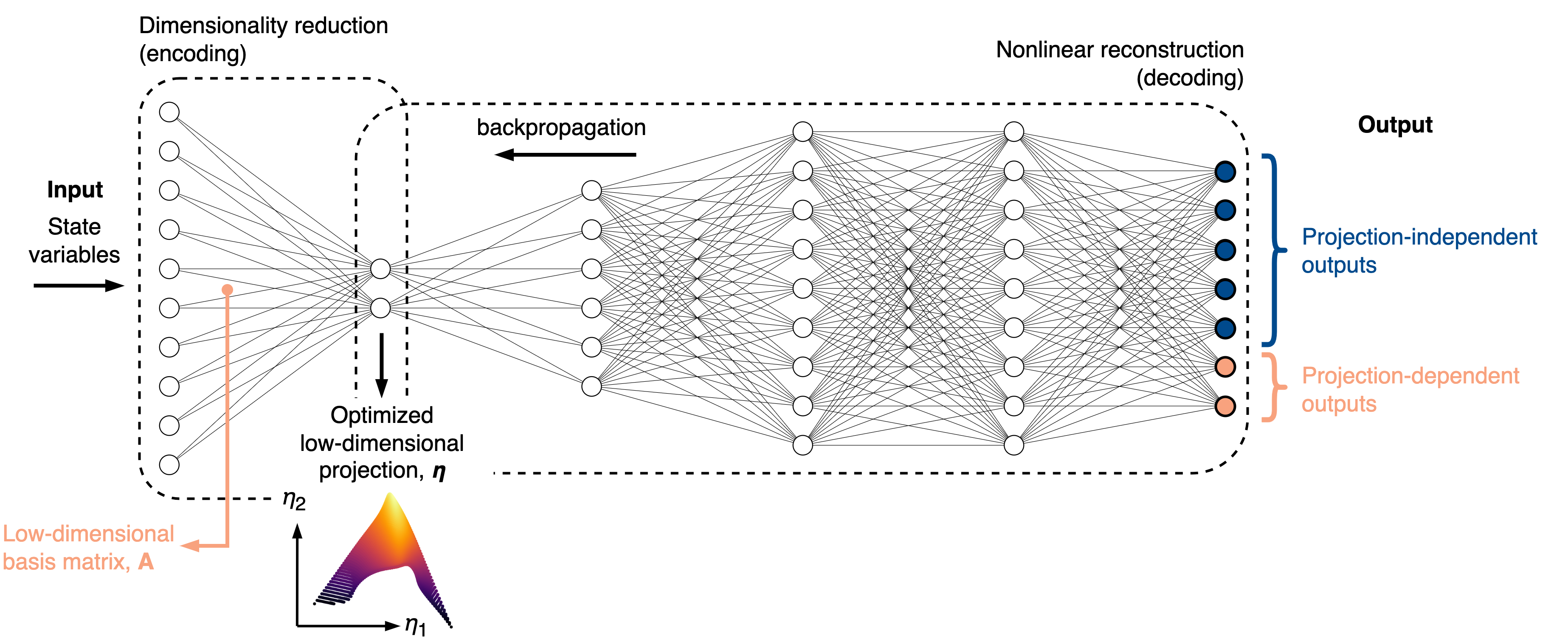
The QoI-aware encoder-decoder is an autoencoder-like neural network that reconstructs important quantities of interest (QoIs) at the output of a decoder. The QoIs can be set to projection-independent variables (such as the original state variables) or projection-dependent variables, whose definition changes during neural network training.
We introduce an intrusive modification to the neural network training process such that at each epoch, a low-dimensional basis matrix is computed from the current weights in the encoder. Any projection-dependent variables at the output get re-projected onto that basis.
The rationale for performing dimensionality reduction with the QoI-aware strategy is that any poor topological behaviors on a low-dimensional projection will immediately increase the loss during training. These behaviors could be non-uniqueness in representing QoIs due to overlaps on a projection, or large gradients in QoIs caused by data compression in certain regions of a projection. Thus, the QoI-aware strategy naturally promotes improved projection topologies and can be useful in reduced-order modeling.
An illustrative explanation of how the QoI-aware encoder-decoder works is presented in the figure below:
More information can be found in [ZdybalPS23].
Example:
from PCAfold import center_scale, QoIAwareProjection
import numpy as np
from tensorflow import optimizers
from tensorflow.keras import initializers

# Generate dummy dataset:
X = np.random.rand(100,8)
S = np.random.rand(100,8)

# Request 2D QoI-aware encoder-decoder projection of the dataset:
n_components = 2

# Preprocess the dataset before passing it to the encoder-decoder:
(input_data, centers, scales) = center_scale(X, scaling='0to1')
projection_dependent_outputs = S / scales

# Instantiate QoIAwareProjection class object:
qoi_aware = QoIAwareProjection(input_data,
                               n_components,
                               optimizer=optimizers.legacy.Adam(learning_rate=0.001),
                               projection_independent_outputs=input_data[:,0:3],
                               projection_dependent_outputs=projection_dependent_outputs,
                               activation_decoder=('tanh', 'tanh', 'linear'),
                               decoder_interior_architecture=(5,8),
                               encoder_weights_init=None,
                               decoder_weights_init=None,
                               encoder_kernel_initializer=initializers.RandomNormal(seed=100),
                               decoder_kernel_initializer=initializers.GlorotUniform(seed=100),
                               trainable_encoder_bias=True,
                               hold_initialization=10,
                               hold_weights=2,
                               transformed_projection_dependent_outputs='signed-square-root',
                               loss='MSE',
                               batch_size=100,
                               n_epochs=200,
                               validation_perc=10,
                               random_seed=100,
                               verbose=True)

# Begin model training:
qoi_aware.train()
A summary of the current QoI-aware encoder-decoder model and its hyperparameter settings can be printed using the
summary()function:# Print the QoI-aware encoder-decoder model summary qoi_aware.summary()
QoI-aware encoder-decoder model summary... (Model has been trained) - - - - - - - - - - - - - - - - - - - - - - - - - - - - - - - - - - - - - - - - - - - - - - - - - - - - - - - - - - - - Projection dimensionality: - 2D projection - - - - - - - - - - - - - - - - - - - - - - - - - - - - - - - - - - - - - - - - - - - - - - - - - - - - - - - - - - - - Encoder-decoder architecture: 8-2-5-8-7 - - - - - - - - - - - - - - - - - - - - - - - - - - - - - - - - - - - - - - - - - - - - - - - - - - - - - - - - - - - - Activation functions: (8)--linear--(2)--tanh--(5)--tanh--(8)--linear--(7) - - - - - - - - - - - - - - - - - - - - - - - - - - - - - - - - - - - - - - - - - - - - - - - - - - - - - - - - - - - - Variables at the decoder output: - 3 projection independent variables - 2 projection dependent variables - 2 transformed projection dependent variables using signed-square-root - - - - - - - - - - - - - - - - - - - - - - - - - - - - - - - - - - - - - - - - - - - - - - - - - - - - - - - - - - - - Model validation: - Using 10% of input data as validation data - Model will be trained on 90% of input data - - - - - - - - - - - - - - - - - - - - - - - - - - - - - - - - - - - - - - - - - - - - - - - - - - - - - - - - - - - - Hyperparameters: - Batch size: 100 - # of epochs: 200 - Optimizer: <keras.src.optimizers.legacy.adam.Adam object at 0x7f9e0f29f310> - Loss function: MSE - - - - - - - - - - - - - - - - - - - - - - - - - - - - - - - - - - - - - - - - - - - - - - - - - - - - - - - - - - - - Weights initialization in the encoder: - Glorot uniform - - - - - - - - - - - - - - - - - - - - - - - - - - - - - - - - - - - - - - - - - - - - - - - - - - - - - - - - - - - - Weights initialization in the decoder: - Glorot uniform - - - - - - - - - - - - - - - - - - - - - - - - - - - - - - - - - - - - - - - - - - - - - - - - - - - - - - - - - - - - Weights updates in the encoder: - Initial weights in the encoder will be kept for 10 first epochs - Weights in the encoder will change once every 2 epochs - - - - - - - - - - - - - - - - - - - - - - - - - - - - - - - - - - - - - - - - - - - - - - - - - - - - - - - - - - - - Results reproducibility: - Reproducible neural network training will be assured using random seed: 100 = = = = = = = = = = = = = = = = = = = = = = = = = = = = = = = = = = = = = = = = = = = = = = = = = = = = = = = = = = = = Training results: - Minimum training loss: 0.0852246955037117 - Minimum training loss at epoch: 199 - Minimum validation loss: 0.06681100279092789 - Minimum validation loss at epoch: 182 - - - - - - - - - - - - - - - - - - - - - - - - - - - - - - - - - - - - - - - - - - - - - - - - - - - - - - - - - - - -- Parameters:
input_data –
numpy.ndarrayspecifying the data set used as the input to the encoder-decoder. It should be of size(n_observations,n_variables). Note that input data is not preprocessed inside theQoIAwareProjectionclass in any way. If the input data should be centered and scaled, you need to take care of this before passing it as a parameter.n_components –
intspecifying the dimensionality of the QoI-aware encoder-decoder projection. This is equal to the number of neurons in the bottleneck layer.optimizer –
tf.optimizersortf.optimizers.legacyorstrspecifying the optimizer to use along with its parameters.projection_independent_outputs – (optional)
numpy.ndarrayspecifying any projection-independent outputs at the decoder. It should be of size(n_observations,n_projection_independent_outputs).projection_dependent_outputs – (optional)
numpy.ndarrayspecifying any projection-dependent outputs at the decoder. During training,projection_dependent_outputsis projected onto the current basis matrix and the decoder outputs are updated accordingly. It should be of size(n_observations,n_variables).activation_decoder – (optional)
strortuplespecifying activation functions in all the decoding layers. If set tostr, the same activation function is used in all decoding layers. If set to atupleofstr, a different activation function can be set at different decoding layers. The number of elements in thetupleshould match the number of decoding layers!strandstrelements of thetuplecan only be'linear','sigmoid', or'tanh'. Note, that the activation function in the encoder is hardcoded to'linear'.decoder_interior_architecture – (optional)
tupleofintspecifying the number of neurons in the interior architecture of a decoder. For example, ifdecoder_interior_architecture=(4,5), two interior decoding layers will be created and the overal network architecture will be(Input)-(Bottleneck)-(4)-(5)-(Output). If set to an empty tuple,decoder_interior_architecture=(), the overal network architecture will be(Input)-(Bottleneck)-(Output). Keep in mind that if you’d like to create just one interior layer, you should use a comma after the integer:decoder_interior_architecture=(4,).encoder_weights_init – (optional)
numpy.ndarrayspecifying the custom initalization of the weights in the encoder. It should be of size(n_variables, n_components). If set toNoneandencoder_kernel_initializeris set toNone, weights in the encoder will be initialized using the Glorot uniform distribution.decoder_weights_init – (optional)
tupleofnumpy.ndarrayspecifying the custom initalization of the weights in the decoder. Each element in the tuple should have a shape that matches the architecture. If set toNoneanddecoder_kernel_initializeris set toNone, weights in the encoder will be initialized using the Glorot uniform distribution.encoder_kernel_initializer – (optional)
tf.keras.initializersspecifying the initialization of the weights in the encoder. Only used whenencoder_weights_initis set toNone. If set toNoneandencoder_weights_initis set toNone, weights in the encoder will be initialized using the Glorot uniform distribution. To assure fully reproducible training, pass a random seed to the initializer, e.g.,tf.keras.initializers.GlorotUniform(seed=100).decoder_kernel_initializer – (optional)
tf.keras.initializersspecifying the initialization of the weights in the decoder. Only used whendecoder_weights_initis set toNone. If set toNoneanddecoder_weights_initis set toNone, weights in the decoder will be initialized using the Glorot uniform distribution. To assure fully reproducible training, pass a random seed to the initializer, e.g.,tf.keras.initializers.GlorotUniform(seed=100).trainable_encoder_bias – (optional)
boolspecifying if the biases in the encoding layer should be trainable. Note, that for linear projections, bias does not change the projection quality and only acts to translate the projection along the low-dimensional coordinates.hold_initialization – (optional)
intspecifying the number of first epochs during which the initial weights in the encoder are held constant. If set toNone, weights in the encoder will change at the first epoch. This parameter can be used in conjunction withhold_weights.hold_weights – (optional)
intspecifying how frequently the weights should be changed in the encoder. For example, if set tohold_weights=2, the weights in the encoder will only be updated once every two epochs throught the whole training process. If set toNone, weights in the encoder will change at every epoch. This parameter can be used in conjunction withhold_initialization.transformed_projection_dependent_outputs – (optional)
strspecifying if any nonlinear transformation of the projection-dependent outputs should be added at the decoder output. It can be'symlog'or'signed-square-root'.transform_power – (optional)
intorfloatas perpreprocess.power_transform().transform_shift – (optional)
intorfloatas perpreprocess.power_transform().transform_sign_shift – (optional)
intorfloatas perpreprocess.power_transform().loss – (optional)
strspecifying the loss function. It can be'MAE'or'MSE'.batch_size – (optional)
intspecifying the batch size.n_epochs – (optional)
intspecifying the number of epochs.validation_perc – (optional)
intspecifying the percentage of the input data to be used as validation data during training. It should be a number larger than or equal to 0 and smaller than 100. Note, that if it is set above 0, not all of the input data will be used as training data. Note, that validation data does not impact model training!random_seed – (optional)
intspecifying the random seed to be used for any random operations. It is highly recommended to set a fixed random seed, as this allows for complete reproducibility of the results.verbose – (optional)
boolfor printing verbose details.
Attributes:
input_data - (read only)
numpy.ndarrayspecifying the data set used as the input to the encoder-decoder.n_components - (read only)
intspecifying the dimensionality of the QoI-aware encoder-decoder projection.projection_independent_outputs - (read only)
numpy.ndarrayspecifying any projection-independent outputs at the decoder.projection_dependent_outputs - (read only)
numpy.ndarrayspecifying any projection-dependent outputs at the decoder.architecture - (read only)
strspecifying the QoI-aware encoder-decoder architecture.n_total_outputs - (read only)
intcounting the total number of outputs at the decoder.qoi_aware_encoder_decoder - (read only) object of
Keras.models.Sequentialclass that stores the QoI-aware encoder-decoder neural network.weights_and_biases_init - (read only)
listofnumpy.ndarrayspecifying weights and biases with which the QoI-aware encoder-decoder was intialized.weights_and_biases_trained - (read only)
listofnumpy.ndarrayspecifying weights and biases after training the QoI-aware encoder-decoder. Only available after callingQoIAwareProjection.train().training_loss - (read only)
listof losses computed on the training data. Only available after callingQoIAwareProjection.train().validation_loss - (read only)
listof losses computed on the validation data. Only available after callingQoIAwareProjection.train()and only whenvalidation_percwas not equal to 0.weights_and_biases_best - (read only)
listofnumpy.ndarrayspecifying all weights and biases corresponding to the epoch at which the training loss was the smallest. Only available after callingQoIAwareProjection.train().
- PCAfold.utilities.QoIAwareProjection.summary(self)
Prints the QoI-aware encoder-decoder model summary.
- PCAfold.utilities.QoIAwareProjection.train(self)
Trains the QoI-aware encoder-decoder neural network model.
After training, the optimized basis matrix for low-dimensional data projection can be obtained.
- PCAfold.utilities.QoIAwareProjection.print_weights_and_biases_init(self)
Prints initial weights and biases from all layers of the QoI-aware encoder-decoder.
- PCAfold.utilities.QoIAwareProjection.print_weights_and_biases_trained(self)
Prints trained weights and biases from all layers of the QoI-aware encoder-decoder.
- PCAfold.utilities.QoIAwareProjection.plot_losses(self, markevery=100, figure_size=(15, 5), save_filename=None)
Plots training and validation losses.
- Parameters:
markevery – (optional)
intspecifying how frequently the epoch number on the x-axis should be labelled.figure_size – (optional)
tuplespecifying figure size.save_filename – (optional)
strspecifying plot save location/filename. If set toNoneplot will not be saved. You can also set a desired file extension, for instance.pdf. If the file extension is not specified, the default is.png.
- Returns:
plt -
matplotlib.pyplotplot handle.
Class QoIAwareProjectionPOUnet
- class PCAfold.utilities.QoIAwareProjectionPOUnet(projection_weights, partition_centers, partition_shapes, basis_type, projection_biases=None, basis_coeffs=None, dtype='float64', **kwargs)
This is analogous to
QoIAwareProjectionbut usesPartitionOfUnityNetworkas the decoder.More information can be found in [AS24].
Example:
from PCAfold import init_uniform_partitions, PCA, QoIAwareProjectionPOUnet
import numpy as np
import tensorflow as tf

# generate dummy data set:
ivars = np.random.rand(100,3)

# initialize a projection (e.g., using PCA)
pca = PCA(ivars, scaling='none', n_components=2)
ivar_proj = pca.transform(ivars)

# initialize the QoIAwareProjectionPOUnet parameters
net = QoIAwareProjectionPOUnet(pca.A[:,:2], **init_uniform_partitions([5,7], ivar_proj), basis_type='linear')

# function for defining the training dependent variables (can include a projection)
dvar = np.vstack((ivars[:,0] + ivars[:,1], 2.*ivars[:,0] + 3.*ivars[:,1], 3.*ivars[:,0] + 5.*ivars[:,1])).T
def dvar_func(proj_weights):
    temp = tf.Variable(np.expand_dims(dvar, axis=2), name='eval_qoi', dtype=net._reconstruction._dtype)
    temp = net.tf_projection(temp, nobias=True)
    return temp

# build the training graph with provided training data
net.build_training_graph(ivars, dvar_func)

# train the projection
net.train(1000)

# compute new projected variables
net.projection(ivars)

# evaluate the encoder-decoder
net(ivars)

# Save the data to a file
net.write_data_to_file('filename.pkl')

# reload projection data from file
net2 = QoIAwareProjectionPOUnet.load_from_file('filename.pkl')
- Parameters:
projection_weights – array of the projection matrix weights
partition_centers – array size (number of partitions) x (number of ivar inputs) for partition locations
partition_shapes – array size (number of partitions) x (number of ivar inputs) for partition shapes influencing the RBF widths
basis_type – string (
'constant','linear', or'quadratic') for the degree of polynomial basisprojection_biases – (optional, default None) array of the biases (offsets) corresponding to the projection weights, if
Nonethe projections are offset by zerosbasis_coeffs – (optional, default
None) if the array of polynomial basis coefficients is known, it may be provided here, otherwise it will be initialized withbuild_training_graphand trained withtraindtype – (optional, default
'float64') string specifying either float type'float64'or'float32'
Attributes:
projection_weights - (read only) array of the current projection weights
projection_biases - (read only) array of the projection biases
reconstruction_model - (read only) the current POUnet decoder
partition_centers - (read only) array of the current partition centers
partition_shapes - (read only) array of the current partition shape parameters
basis_type - (read only) string relaying the basis degree
basis_coeffs - (read only) array of the current basis coefficients
proj_ivar_center - (read only) array of the centering parameters used in the POUnet for the projected ivar inputs
proj_ivar_scale - (read only) array of the scaling parameters used in the POUnet for the projected ivar inputs
dtype - (read only) string relaying the data type (
'float64'or'float32')training_archive - (read only) dictionary of the errors and POUnet states archived during training
iterations - (read only) array of the iterations archived during training
- PCAfold.utilities.QoIAwareProjectionPOUnet.projection(self, ivars, nobias=False)
Projects the independent variable inputs using the current projection weights and biases
- Parameters:
ivars – array of independent variable query points
nobias – (optional, default False) whether or not to apply the projection bias. Analogous to
nocenterin the PCAtransformfunction.
- Returns:
array of the projected independent variable query points
- PCAfold.utilities.QoIAwareProjectionPOUnet.tf_projection(self, y, nobias=False)
version of
projectionusing tensorflow operations and Tensors
- PCAfold.utilities.QoIAwareProjectionPOUnet.update_lr(self, lr)
update the learning rate for training
- Parameters:
lr – float for the learning rate
- PCAfold.utilities.QoIAwareProjectionPOUnet.update_l2reg(self, l2reg)
update the least-squares regularization for training
- Parameters:
l2reg – float for the least-squares regularization
- PCAfold.utilities.QoIAwareProjectionPOUnet.build_training_graph(self, ivars, dvars_function, error_type='abs', constrain_positivity=False, first_trainable_idx=0)
Construct the graph used during training (including defining the training errors) with the provided training data
- Parameters:
ivars – array of independent variables for training
dvars_function – function (using tensorflow operations) for defining the dependent variable(s) for training. This must take a single argument of the projection weights which, if used, will be evaluated with the weights as they are updated
error_type – (optional, default
'abs') the type of training error: relative'rel'or absolute'abs'constrain_positivity – (optional, default False) when True, it penalizes the training error with \(f - |f|\) for dependent variables \(f\). This can be useful for defining projected source term dependent variables, for example.
first_trainable_idx – (optional, default 0) This separates the trainable projection weights (with index greater than or equal to
first_trainable_idx) from the nontrainable projection weights.
- PCAfold.utilities.QoIAwareProjectionPOUnet.train(self, iterations, archive_rate=100, use_best_archive_sse=True, verbose=False)
Performs training using a least-squares gradient descent block coordinate descent strategy. This alternates between updating the partition and projection parameters with gradient descent and updating the basis coefficients with least-squares.
- Parameters:
iterations – integer for number of training iterations to perform
archive_rate – (optional, default 100) the rate at which the errors and parameters are archived during training. These can be accessed with the
training_archiveattributeuse_best_archive_sse – (optional, default True) when True will set the POUnet parameters to those with the lowest error observed during training, otherwise the parameters from the last iteration are used
verbose – (optional, default False) when True will print progress
- PCAfold.utilities.QoIAwareProjectionPOUnet.__call__(self, xeval)
evaluate the encoder-decoder
- Parameters:
xeval – array of independent variable query points
- Returns:
array of predictions
- PCAfold.utilities.QoIAwareProjectionPOUnet.write_data_to_file(self, filename)
Save class data to a specified file using pickle. This does not include the archived data from training, which can be separately accessed with training_archive and saved outside of
QoIAwareProjectionPOUnet.- Parameters:
filename – string
- PCAfold.utilities.QoIAwareProjectionPOUnet.load_data_from_file(filename)
Load data from a specified
filenamewith pickle (followingwrite_data_to_file)- Parameters:
filename – string
- Returns:
dictionary of the encoder-decoder data
- PCAfold.utilities.QoIAwareProjectionPOUnet.load_from_file(filename)
Load class from a specified
filenamewith pickle (followingwrite_data_to_file)- Parameters:
filename – string
- Returns:
QoIAwareProjectionPOUnet
Manifold-informed feature selection
- PCAfold.utilities.manifold_informed_forward_variable_addition(X, X_source, variable_names, scaling, bandwidth_values, target_variables=None, add_transformed_source=True, target_manifold_dimensionality=3, bootstrap_variables=None, penalty_function=None, power=1, vertical_shift=1, norm='max', integrate_to_peak=False, verbose=False)
Manifold-informed feature selection algorithm based on forward variable addition introduced in [ZdybalSP22]. The goal of the algorithm is to select a meaningful subset of the original variables such that undesired behaviors on a PCA-derived manifold of a given dimensionality are minimized. The algorithm uses the cost function, \(\mathcal{L}\), based on minimizing the area under the normalized variance derivatives curves, \(\hat{\mathcal{D}}(\sigma)\), for the selected \(n_{dep}\) dependent variables (as per
analysis.cost_function_normalized_variance_derivativefunction). The algorithm can be bootstrapped in two ways:Automatic bootstrap when
bootstrap_variables=None: the first best variable is selected automatically as the one that gives the lowest cost.User-defined bootstrap when
bootstrap_variablesis set to a user-defined list of the bootstrap variables.
The algorithm iterates, adding a new variable that exhibits the lowest cost at each iteration. The original variables in a data set get ordered according to their effect on the manifold topology. Assuming that the original data set is composed of \(Q\) variables, the first output is a list of indices of the ordered original variables, \(\mathbf{X} = [X_1, X_2, \dots, X_Q]\). The second output is a list of indices of the selected subset of the original variables, \(\mathbf{X}_S = [X_1, X_2, \dots, X_n]\), that correspond to the minimum cost, \(\mathcal{L}\).
More information can be found in [ZdybalSP22].
Note
The algorithm can be very expensive (for large data sets) due to multiple computations of the normalized variance derivative. Try running it on multiple cores or on a sampled data set.
In case the algorithm breaks when not being able to determine the peak location, try increasing the range in the
bandwidth_valuesparameter.Example:
from PCAfold import manifold_informed_forward_variable_addition as FVA
import numpy as np

# Generate dummy data set:
X = np.random.rand(100,10)
X_source = np.random.rand(100,10)

# Define original variables to add to the optimization:
target_variables = X[:,0:3]

# Specify variables names
variable_names = ['X_' + str(i) for i in range(0,10)]

# Specify the bandwidth values to compute the optimization on:
bandwidth_values = np.logspace(-4, 2, 50)

# Run the subset selection algorithm:
(ordered, selected, min_cost, costs) = FVA(X,
                                           X_source,
                                           variable_names,
                                           scaling='auto',
                                           bandwidth_values=bandwidth_values,
                                           target_variables=target_variables,
                                           add_transformed_source=True,
                                           target_manifold_dimensionality=2,
                                           bootstrap_variables=None,
                                           penalty_function='peak',
                                           power=1,
                                           vertical_shift=1,
                                           norm='max',
                                           integrate_to_peak=True,
                                           verbose=True)
- Parameters:
X –
numpy.ndarrayspecifying the original data set, \(\mathbf{X}\). It should be of size(n_observations,n_variables).X_source –
numpy.ndarrayspecifying the source terms, \(\mathbf{S_X}\), corresponding to the state-space variables in \(\mathbf{X}\). This parameter is applicable to data sets representing reactive flows. More information can be found in [SP09]. It should be of size(n_observations,n_variables).variable_names –
listofstrspecifying variables names.scaling – (optional)
strspecifying the scaling methodology. It can be one of the following:'none','','auto','std','pareto','vast','range','0to1','-1to1','level','max','poisson','vast_2','vast_3','vast_4'.bandwidth_values –
numpy.ndarrayspecifying the bandwidth values, \(\sigma\), for \(\hat{\mathcal{D}}(\sigma)\) computation.target_variables – (optional)
numpy.ndarrayspecifying the dependent variables that should be used in \(\hat{\mathcal{D}}(\sigma)\) computation. It should be of size(n_observations,n_target_variables).add_transformed_source – (optional)
boolspecifying if the PCA-transformed source terms of the state-space variables should be added in \(\hat{\mathcal{D}}(\sigma)\) computation, alongside the user-defined dependent variables.target_manifold_dimensionality – (optional)
intspecifying the target dimensionality of the PCA manifold.bootstrap_variables – (optional)
listspecifying the user-selected variables to bootstrap the algorithm with. If set toNone, automatic bootstrapping is performed.penalty_function – (optional)
strspecifying the weighting applied to each area. Setpenalty_function='peak'to weight each area by the rightmost peak location, \(\sigma_{peak, i}\), for the \(i^{th}\) dependent variable. Setpenalty_function='sigma'to weight each area continuously by the bandwidth. Setpenalty_function='log-sigma-over-peak'to weight each area continuously by the \(\log_{10}\) -transformed bandwidth, normalized by the right most peak location, \(\sigma_{peak, i}\). Ifpenalty_function=None, the area is not weighted.power – (optional)
floatorintspecifying the power, \(r\). It can be used to control how much penalty should be applied to variance happening at the smallest length scales.vertical_shift – (optional)
floatorintspecifying the vertical shift multiplier, \(b\). It can be used to control how much penalty should be applied to feature sizes.norm – (optional)
strspecifying the norm to apply for all areas \(A_i\).norm='cumulative'uses the \(L_{1}\) norm,norm='average'uses an arithmetic average,norm='L2'uses the \(L_{2}\) norm,norm='normalized-L2'uses the \(L_{2}\) norm divided by the number of target variables,norm='max'uses the \(L_{\infty}\) norm,norm='min'uses a minimum area, andnorm='median'uses a median area.integrate_to_peak – (optional)
boolspecifying whether an individual area for the \(i^{th}\) dependent variable should be computed only up the the rightmost peak location.verbose – (optional)
boolfor printing verbose details.
- Returns:
ordered_variables -
listspecifying the indices of the ordered variables.selected_variables -
listspecifying the indices of the selected variables that correspond to the minimum cost \(\mathcal{L}\).optimized_cost -
floatspecifying the cost corresponding to the optimized subset.costs -
listspecifying the costs, \(\mathcal{L}\), from each iteration.
- PCAfold.utilities.manifold_informed_backward_variable_elimination(X, X_source, variable_names, scaling, bandwidth_values, target_variables=None, add_transformed_source=True, source_space=None, target_manifold_dimensionality=3, penalty_function=None, power=1, vertical_shift=1, norm='max', integrate_to_peak=False, verbose=False)
Manifold-informed feature selection algorithm based on backward variable elimination introduced in [ZdybalSP22]. The goal of the algorithm is to select a meaningful subset of the original variables such that undesired behaviors on a PCA-derived manifold of a given dimensionality are minimized. The algorithm uses the cost function, \(\mathcal{L}\), based on minimizing the area under the normalized variance derivatives curves, \(\hat{\mathcal{D}}(\sigma)\), for the selected \(n_{dep}\) dependent variables (as per
analysis.cost_function_normalized_variance_derivativefunction).The algorithm iterates, removing another variable that has an effect of decreasing the cost the most at each iteration. The original variables in a data set get ordered according to their effect on the manifold topology. Assuming that the original data set is composed of \(Q\) variables, the first output is a list of indices of the ordered original variables, \(\mathbf{X} = [X_1, X_2, \dots, X_Q]\). The second output is a list of indices of the selected subset of the original variables, \(\mathbf{X}_S = [X_1, X_2, \dots, X_n]\), that correspond to the minimum cost, \(\mathcal{L}\).
More information can be found in [ZdybalSP22].
Note
The algorithm can be very expensive (for large data sets) due to multiple computations of the normalized variance derivative. Try running it on multiple cores or on a sampled data set.
In case the algorithm breaks when not being able to determine the peak location, try increasing the range in the
bandwidth_valuesparameter.Example:
from PCAfold import manifold_informed_backward_variable_elimination as BVE
import numpy as np

# Generate dummy data set:
X = np.random.rand(100,10)
X_source = np.random.rand(100,10)

# Define original variables to add to the optimization:
target_variables = X[:,0:3]

# Specify variables names
variable_names = ['X_' + str(i) for i in range(0,10)]

# Specify the bandwidth values to compute the optimization on:
bandwidth_values = np.logspace(-4, 2, 50)

# Run the subset selection algorithm:
(ordered, selected, min_cost, costs) = BVE(X,
                                           X_source,
                                           variable_names,
                                           scaling='auto',
                                           bandwidth_values=bandwidth_values,
                                           target_variables=target_variables,
                                           add_transformed_source=True,
                                           source_space=None,
                                           target_manifold_dimensionality=2,
                                           penalty_function='peak',
                                           power=1,
                                           vertical_shift=1,
                                           norm='max',
                                           integrate_to_peak=True,
                                           verbose=True)
- Parameters:
X –
numpy.ndarrayspecifying the original data set, \(\mathbf{X}\). It should be of size(n_observations,n_variables).X_source –
numpy.ndarrayspecifying the source terms, \(\mathbf{S_X}\), corresponding to the state-space variables in \(\mathbf{X}\). This parameter is applicable to data sets representing reactive flows. More information can be found in [SP09]. It should be of size(n_observations,n_variables).variable_names –
listofstrspecifying variables names. Order of names in thevariable_nameslist should match the order of variables (columns) inX.scaling – (optional)
strspecifying the scaling methodology. It can be one of the following:'none','','auto','std','pareto','vast','range','0to1','-1to1','level','max','poisson','vast_2','vast_3','vast_4'.bandwidth_values –
numpy.ndarrayspecifying the bandwidth values, \(\sigma\), for \(\hat{\mathcal{D}}(\sigma)\) computation.target_variables – (optional)
numpy.ndarrayspecifying the dependent variables that should be used in \(\hat{\mathcal{D}}(\sigma)\) computation. It should be of size(n_observations,n_target_variables).add_transformed_source – (optional)
boolspecifying if the PCA-transformed source terms of the state-space variables should be added in \(\hat{\mathcal{D}}(\sigma)\) computation, alongside the user-defined dependent variables.source_space – (optional)
strspecifying the space to which the PC source terms should be transformed before computing the cost. It can be one of the following:symlog,continuous-symlog,original-and-symlog,original-and-continuous-symlog. If set toNone, PC source terms are kept in their original PCA-space.target_manifold_dimensionality – (optional)
intspecifying the target dimensionality of the PCA manifold.penalty_function – (optional)
strspecifying the weighting applied to each area. Setpenalty_function='peak'to weight each area by the rightmost peak location, \(\sigma_{peak, i}\), for the \(i^{th}\) dependent variable. Setpenalty_function='sigma'to weight each area continuously by the bandwidth. Setpenalty_function='log-sigma-over-peak'to weight each area continuously by the \(\log_{10}\) -transformed bandwidth, normalized by the right most peak location, \(\sigma_{peak, i}\). Ifpenalty_function=None, the area is not weighted.power – (optional)
floatorintspecifying the power, \(r\). It can be used to control how much penalty should be applied to variance happening at the smallest length scales.vertical_shift – (optional)
floatorintspecifying the vertical shift multiplier, \(b\). It can be used to control how much penalty should be applied to feature sizes.norm – (optional)
strspecifying the norm to apply for all areas \(A_i\).norm='cumulative'uses the \(L_{1}\) norm,norm='average'uses an arithmetic average,norm='L2'uses the \(L_{2}\) norm,norm='normalized-L2'uses the \(L_{2}\) norm divided by the number of target variables,norm='max'uses the \(L_{\infty}\) norm,norm='min'uses a minimum area, andnorm='median'uses a median area.integrate_to_peak – (optional)
boolspecifying whether an individual area for the \(i^{th}\) dependent variable should be computed only up the the rightmost peak location.verbose – (optional)
boolfor printing verbose details.
- Returns:
ordered_variables -
listspecifying the indices of the ordered variables.selected_variables -
listspecifying the indices of the selected variables that correspond to the minimum cost \(\mathcal{L}\).optimized_cost -
floatspecifying the cost corresponding to the optimized subset.costs -
listspecifying the costs, \(\mathcal{L}\), from each iteration.