Note

This tutorial was generated from a Jupyter notebook that can be accessed here.

Local feature size estimation

In this tutorial, we present the local feature size estimation tool from the analysis module.

We import the necessary modules:

from PCAfold import preprocess
from PCAfold import reduction
from PCAfold import analysis
import numpy as np
import pandas as pd
import time
import matplotlib
import matplotlib.pyplot as plt

and we set some initial parameters:

save_filename = None
bandwidth_values = np.logspace(-5, 1, 40)

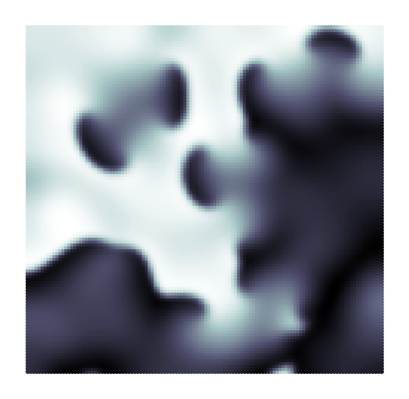
We upload the dataset which comes from solving the Brusselator PDE. The datasets has two independent variables, \(x\) and \(y\), and one dependent variable, \(\phi\). The dataset is generated on a uniform \(x\)-\(y\) grid.

data = pd.read_csv('brusselator-PDE.csv', header=None).to_numpy()
indepvars = data[:,0:2]
depvar = data[:,2:3]

---

Compute the feature sizes map on a synthetic dataset

We start by computing the normalized variance, \(\hat{\mathcal{N}}(\sigma)\). In order to compute the quantities necessary for drawing the feature size map, we need to set either compute_sample_norm_var=True or compute_sample_norm_range=True.

tic = time.perf_counter()

variance_data = analysis.compute_normalized_variance(indepvars,
                                                     depvars=depvar,
                                                     depvar_names=['phi'],
                                                     bandwidth_values=bandwidth_values,
                                                     compute_sample_norm_range=True)

toc = time.perf_counter()
print(f'\tTime it took: {(toc - tic)/60:0.1f} minutes.\n' + '-'*40)

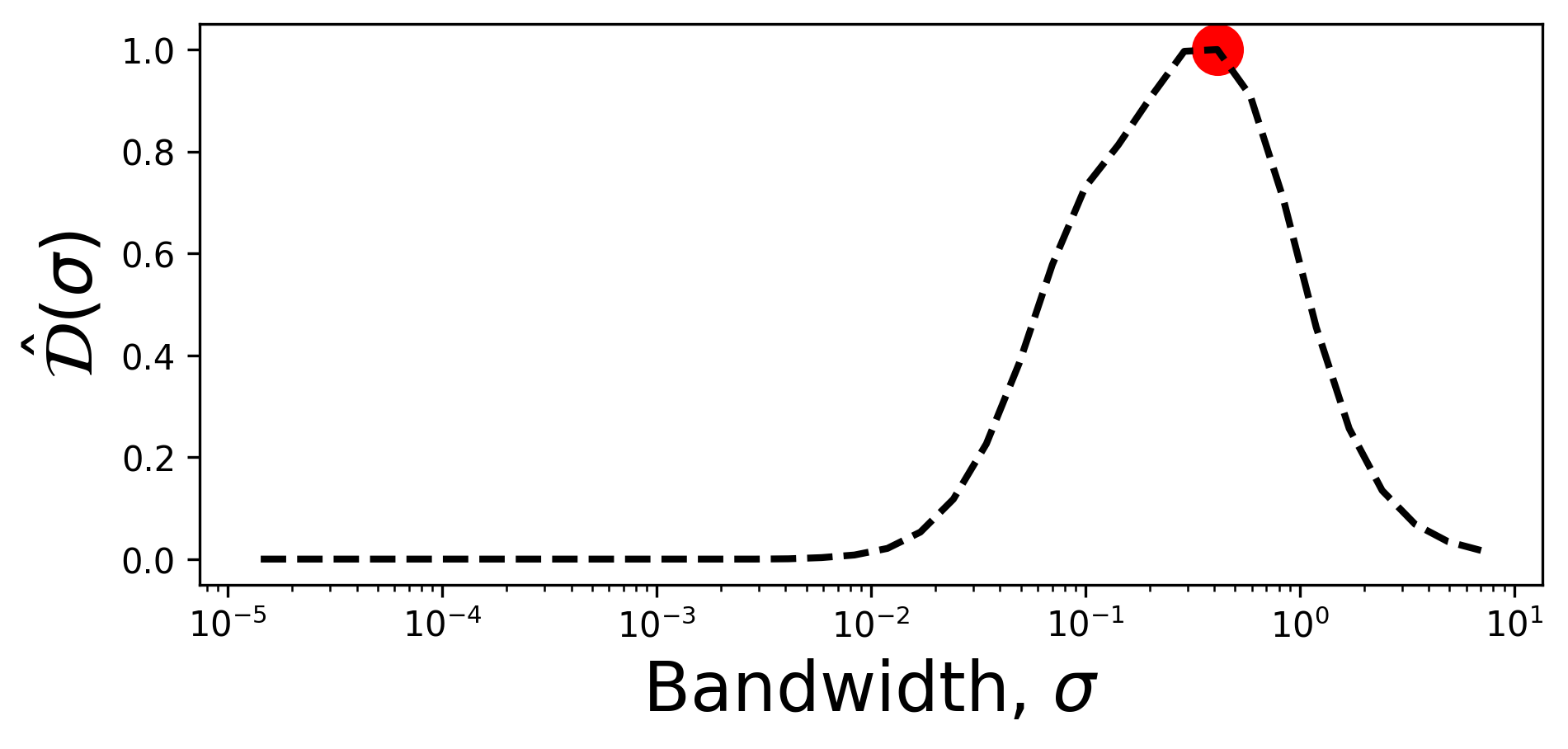
We compute the normalized variance derivative, \(\hat{\mathcal{D}}(\sigma)\):

derivative, sigmas, _ = analysis.normalized_variance_derivative(variance_data)
derivatives = derivative['phi']

The local feature size estimation algorithm iteratively updates the size of the local features by running “bandwidth descent” algorithm. The goal is to compute the bandwidth vector \(\mathbf{B}\) which contains estimation of the local feature size tied to every data point. The vector \(\mathbf{B}\) is first initialized with the largest feature sizes indicated by the starting_bandwidth_idx parameter. Entries in \(\mathbf{B}\) are iteratively updated based on the cutoff value.

starting_bandwidth_idx = 29

We run bandwidth descent algorithm. This will update the bandwidth vector at each location where the sample normalized variance is above cutoff of its maximum value.

cutoff = 15

B = analysis.feature_size_map(variance_data,
                              variable_name='phi',
                              cutoff=cutoff,
                              starting_bandwidth_idx='peak',
                              use_variance=False,
                              verbose=True)